1. Why these updates are connected
A generator produces a distribution of outputs. Suppose we want that distribution to match a target. A divergence measures the mismatch:
First choose what to match. Distillation uses a teacher distribution; GANs use the real data distribution. In KL-regularized RL, reward reshapes a reference distribution, giving higher-reward outputs more weight. Each specifies a target in a different way.
Next choose how to measure the mismatch. We will use reverse KL. With a suitable adversarial loss, GAN training can optimize this same divergence toward real data.
Finally choose how to compute the update. Evaluating probabilities lets us reward sampled outputs. Differentiating through outputs lets us move them toward lower loss. For Gaussian predictions with the same fixed variance, averaging the sampling noise gives a mean-squared-error gradient.
Choose the target, choose the divergence, then choose how to differentiate it.
We will follow these choices to connect policy gradients (REINFORCE / GRPO), On-Policy Distillation (OPD), Gaussian mean matching (DiffusionOPD), and sample movement using diffusion scores (VSD / DMD) or a discriminator (GAN).
Our working example: reverse KL to a chosen target.
Weight sampled actions
01Estimate the policy gradient.
Compute KL directly → mean MSE.
Move generated outputs
03Estimate two density scores.
Differentiate a discriminator logit.
Notation: \(q_\theta\) is the student distribution, \(p_T\) the teacher, and \(p\) a fixed target. We hold the prompt fixed and assume the KLs and gradients are well-defined.
2. RL: improve the policy through a scalar reward
For a complete output \(x\) and fixed reward \(r(x)\), optimize the policy \(q_\theta\) to increase expected reward:
This is REINFORCE: sample outputs from the policy and use their rewards to weight the log-probability gradients. [1]
3. OPD: a teacher supplies an implicit reward
In On-Policy Distillation, the student generates responses and the teacher evaluates them. [2] Treat each complete response as one sample, and choose reverse KL between their distributions:
Negate the loss to align with RL's maximization convention:
The teacher supplies the reward: \(\log p_T(x)-\log q_\theta(x)\). It is positive when the teacher assigns an output more probability than the student does.
The reward depends on \(\theta\), but its extra derivative averages to zero by the same normalization identity used in (2). In the sampled policy-gradient update, we therefore treat the reward as a fixed weight.
Token rewards, discounting, and practical OPD
For the full-response KL above, an early token affects the rest of the response. Its update therefore includes later rewards. Let \(h_k\) be the prefix before \(y_k\), and \(H\) the maximum response length including EOS; rewards after EOS are zero:
The weight \(\hat A_k=R_k-b(h_k)\) is an advantage estimate: how much better or worse this continuation is than a reference score \(b(h_k)\). For example, return 8 against baseline 5 gives advantage \(+3\).
PPO learns a value function, or critic, to predict the remaining return and help estimate advantages. Its clipped surrogate objective weights new/old policy probability ratios by these advantages, limiting the incentive for large policy changes. [4]
GRPO keeps clipped policy optimization but replaces the learned critic with comparisons among responses to the same prompt. For outcome rewards, it subtracts the group's mean reward and divides by its standard deviation. [15]
Why is there no discount in (4)?
A discounted return would be
\(\gamma=1\) counts every later reward; \(\gamma=0\) keeps only the current reward. To see why the full-response KL uses \(\gamma=1\), write the probability of a response \(y=(y_1,\ldots,y_H)\) as a product:
Taking a log turns the product into a sum. Every token has weight one, so no discount appears. The same identity applied to the remaining response gives \(R_k\).
In practice, Thinking Machines Lab's OPD explicitly sets \(\gamma=0\). Each token's log-ratio \(r_k\) goes directly into the training code's advantages field. The authors report no improvement from including future rewards. [16]
4. KL-regularized RL defines a target distribution
In KL-regularized RL, we reward good outputs while keeping the policy close to a reference. For fixed reward \(r\), reference \(p_{\rm ref}\), and strength \(\beta>0\):
The target \(p^*\) is the reference distribution reweighted by reward. Substituting its log probability into KL gives
KL-regularized RL is reverse-KL matching to a reward-weighted target. The term \(\beta\log Z\) is constant, so it does not affect the update. Choosing this target as the teacher makes the two objectives equivalent up to scale and a constant. [5]
5. Gaussian OPD: KL is mean MSE
For Gaussian predictions with the same fixed variance, KL already has a closed form. Fix the input, the teacher mean \(\mu_T\), and the shared noise scale \(\sigma>0\):
This gives a simple training objective: minimize the squared difference between the two means. We revisit policy gradient below to show that averaging its sampling noise recovers this same analytic gradient.
The same gradient from policy gradient
Equation (2) writes the KL gradient as \(\mathbb E[c_\theta(a)\nabla_\theta\log q_\theta(a)]\), where \(c_\theta=\log q_\theta-\log p_T\) is the log-ratio cost. Sample a Gaussian action:
Substitute the sampled action into the log ratio, and compute the log-probability gradient with the action held fixed:
Multiply them and use \(\mathbb E[\epsilon]=0\), \(\mathbb E[\epsilon\epsilon^{\mathsf T}]=I\):
One KL objective, two ways to compute its gradient. Direct differentiation of mean MSE gives the result immediately; the policy-gradient calculation explains its connection to OPD.
From transition means to diffusion predictions
In diffusion, apply this argument to the next-step prediction at a fixed sampled state. DiffusionOPD and Flow-OPD use Gaussian transition KL to obtain a weighted MSE between student and teacher predictions, then differentiate this loss directly. [10] [11]
If the transition mean is \(\mu_\theta(h,t)=b(h,t)+k(t)v_\theta(h,t)\), with shared fixed \(b,k,\sigma_t\), matching means becomes matching model predictions:
This MSE matches one prediction at a fixed input. For a deterministic ODE step, direct MSE is a regression objective; the Gaussian KL derivation requires positive transition noise.
6. From rewarding samples to moving samples
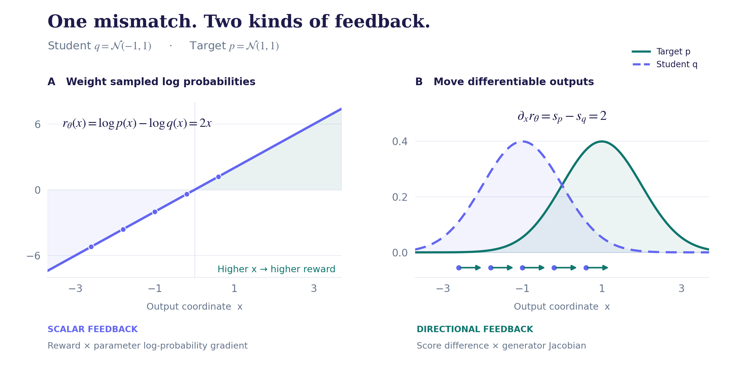
In OPD, the log ratio tells us which outputs should become more likely. The Gaussian example showed that the same KL gradient can also be computed by directly adjusting the mean. Can we extend this idea to a continuous generator whose output distribution is not Gaussian?
Its KL may have no closed form, but we can differentiate through the generated sample. Keep the reverse-KL objective from Equation (2), with \(p\) as the fixed target, and write sampling as a differentiable function of random input \(z\):
This is reparameterization: changing \(\theta\) moves the sample \(x\), while the distribution of \(z\) stays fixed. Assume smooth positive densities, and define their scores as \(s_q=\nabla_x\log q_\theta\) and \(s_p=\nabla_x\log p\). Rewrite KL using \(x=G_\theta(z)\), then apply the chain rule:
The extra term vanishes by normalization, just as in Equation (2). To reduce KL, backpropagate the target-minus-student score difference through the generator:
The log ratio tells us how to weight an output; its gradient tells us where to move it. For the same smooth continuous model, OPD's policy gradient and this sample-based calculation give the same expected parameter gradient. VSD / DMD and discriminator-based updates provide ways to estimate this movement direction, as we will see next.
Vector PDFFigure source
Watch the updates
7. VSD / DMD: match noisy marginals
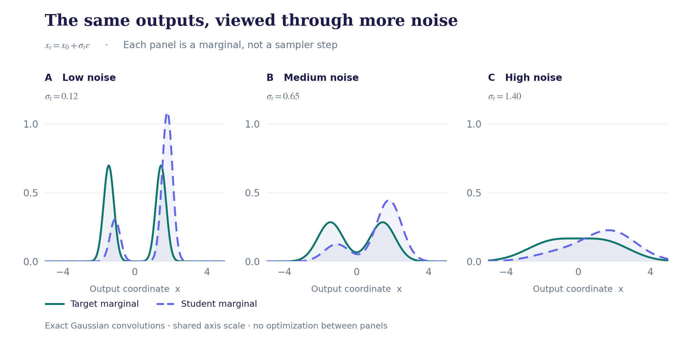
VSD / DMD apply the same KL-to-score calculation at multiple noise levels. Add the same Gaussian noise process to generated and target images, giving distributions \(q_{\theta,t}\) and \(p_{T,t}\):
Vector PDFFigure source
Apply Equation (7) at each noise level. With \(s_{q,t}=\nabla_{x_t}\log q_{\theta,t}\), \(s_{T,t}=\nabla_{x_t}\log p_{T,t}\), and \(\partial_\theta x_t=\alpha_tJ_\theta\):
The teacher supplies the target score; an auxiliary denoiser trained on student outputs estimates the student score. VSD backpropagates their difference through a renderer to optimize 3D scenes; DMD backpropagates through an image generator. [6] [7] [8]
For the full derivation, see From a Marginal KL to Two Scores. For score estimation and the additional losses used by DMD / DMD2, see What SDS, VSD, and DMD Actually Estimate. [9]
8. GANs: learn the ratio, then differentiate it
VSD / DMD obtain a direction for moving samples from two score estimates. A GAN discriminator offers another route: learn the log ratio from real and generated examples, then differentiate it to obtain the score difference in Equation (8).
Start with the original minimax GAN losses. The discriminator \(D_\psi\) classifies real samples from \(p\) and generated samples from \(q_\theta\), with equal class weights; the generator tries to fool it: [12]
For a fixed generator, the optimal classifier is \(D^*=p/(p+q_\theta)\). Its logit, \(f=\log[D/(1-D)]\), therefore gives the log ratio:
We can now read the generator update from the same score perspective as VSD / DMD. Freeze the discriminator's parameters and differentiate through its input. Since \(D=\operatorname{sigmoid}(f)\):
At the optimal discriminator for the current generator, substitute Equation (12) and backpropagate through \(x=G_\theta(z)\). Under the smooth-density assumptions from Section 6, we obtain:
Keep the same discriminator training, but change the generator loss to the negative logit. Its derivative removes the \(D(x)\) factor:
Both updates move samples using the same score difference; the generator loss determines the weight. At the ideal current discriminator, the weighted form corresponds to the gradient of \(2\,\mathrm{JS}(p\|q_\theta)\), as follows from the original GAN's minimax result, while the unweighted form recovers the reverse-KL gradient in Equation (8). [12, §4.1]
9. Implementation: where gradients flow
The examples below implement OPD's reward-weighted update, VSD / DMD's score-based update, and GAN's discriminator-based update.
Three short gradient examples
Policy gradient
# x is sampled from exactly q_theta, with no sampling gradient.
# Sum response-token log probabilities, including EOS; mask padding.
logq = student_log_prob(x)
logp = teacher_log_prob(x)
reward = (logp - logq).detach()
loss_pg = -(reward * logq).mean()
loss_pg.backward()
Sample from the current student. Use the full response log probabilities and detach the reward weight.
Score distillation
# Generator update: both score estimates are evaluated, then detached.
x0 = generator(z)
xt = alpha * x0 + sigma * noise
with no_grad():
    grad_xt = w * (fake_score(xt, t) - teacher_score(xt, t))
loss_dm = (grad_xt * xt).flatten(1).sum(1).mean()
loss_dm.backward()  # d xt / d theta supplies alpha * the generator Jacobian
Train the auxiliary denoiser separately. During the generator update, detach the score difference and backpropagate through \(x_t\). The code supplies the KL gradient, not its scalar value.
Discriminator feedback
# Generator step: freeze discriminator parameters, keep its input gradient.
discriminator.eval()
for parameter in discriminator.parameters():
    parameter.requires_grad_(False)
x = generator(z)
loss_ratio = -discriminator.logit(x).mean()
loss_ratio.backward()  # backpropagate through discriminator INTO x
# Restore training mode and parameter gradients for the discriminator update.
Freeze discriminator parameters, but keep its input gradient so the generator receives the update.
10. A compact map of the connection
| View | Training signal | Update |
|---|---|---|
| Policy gradient / discrete OPD | External reward or teacher–student log ratio | Weight \(\nabla_\theta\log q_\theta\) by a scalar return |
| Gaussian OPD | Local KL with shared fixed covariance | Analytic mean-MSE gradient |
| VSD / DMD | Scores of noisy output distributions | Backpropagate a two-score field |
| GAN / discriminator | A learned log-density ratio | Backpropagate the logit, weighted by the generator loss |
For a new method, ask which distribution it compares, which loss it minimizes, and how it computes the gradient.
Numerical checks cover sequence gradients, Gaussian PG-to-MSE, entropy, noisy scores, and GAN losses using quadrature and finite differences.
References
- [1]
- [2]
- [3]
- [4]
- [5]
- [6]
- [7]
- [8]
- [9]
- [10]
- [11]
- [12]
- [13]
- [14]
- [15]
- [16]