Distributional Distillation III: From Scores to Flows

From the Part I identity to distributional flows

How a distributional gradient becomes a particle direction
Why Wasserstein-2 selects \(-\nabla\delta\mathcal F/\delta q\)
Why detached regression implements the same local update
DMD as KL gradient flow on noisy marginals
Drifting Models through the KDE–score connection
How W-Flow changes the batch interaction

1. From a distributional objective to a particle direction

What we are reusing from Part I Part I already proved the identity that converts density motion into particle motion. We repeat it here because we now want to read every factor operationally: sample a particle, compute the direction in which it should move, and pass that request back through the generator.

We sample a latent \(\mathbf z\), pass it through the generator, and call the resulting output distribution \(q_\theta\):

\[ \mathbf x_\theta=f_\theta(\mathbf z), \qquad q_\theta=(f_\theta)_\#p_{\mathrm{ref}}, \qquad J_\theta=\frac{\partial f_\theta(\mathbf z)}{\partial\theta}. \]

Let the scalar \(\mathcal F_p(q)\) grade the whole generated distribution against a target \(p\). Its first variation turns that one global number into a scalar field over sample space: if we add or remove a tiny amount of probability near \(\mathbf x\), how does the objective change?

\[ \phi_q(\mathbf x) \equiv \frac{\delta\mathcal F_p}{\delta q}(q)(\mathbf x). \]

We call this local sensitivity \(\phi_q(\mathbf x)\). Part I showed that, after evaluating this field at the current distribution and holding it fixed for the first-order step, the functional chain rule can be rewritten in terms of generated particles:

\[ \begin{aligned} \nabla_\theta\mathcal F_p(q_\theta) &=\int\nabla_\theta q_\theta(\mathbf x) \phi_{q_\theta}(\mathbf x)d\mathbf x\\ &=\mathbb E_{\mathbf z}\!\left[ J_\theta^\top \nabla_{\mathbf x}\phi_{q_\theta}(\mathbf x_\theta) \right]. \end{aligned} \] (1)

Now we can read the last line particle by particle. At a sampled point \(\mathbf x\), the spatial gradient \(\nabla_{\mathbf x}\phi_q(\mathbf x)\) points in the direction in which moving that particle would increase the objective to first order. Therefore the requested descent direction is its negative:

\[ \boldsymbol\xi_q(\mathbf x) \equiv-\nabla_{\mathbf x}\phi_q(\mathbf x). \]

If particles were free to move independently, one local optimization step would simply be

\[ \mathbf x \leftarrow \mathbf x+\eta\boldsymbol\xi_q(\mathbf x) =\mathbf x-\eta\nabla_{\mathbf x}\phi_q(\mathbf x). \]

This gives the promised particle interpretation of distributional optimization: sample particles from \(q\), evaluate a direction at each particle, and move them along that direction. A neural generator cannot move its samples independently because they share parameters, so the Jacobian \(J_\theta\) pulls all of these particle-level requests back to one parameter gradient. Equation (1) becomes

\[ \boxed{ \mathcal F_p(q) \longrightarrow \phi_q=\frac{\delta\mathcal F_p}{\delta q} \xrightarrow{\text{particle descent}} \boldsymbol\xi_q=-\nabla\phi_q \longrightarrow \nabla_\theta\mathcal F_p(q_\theta) =-\mathbb E[J_\theta^\top\boldsymbol\xi_q].} \] (2)

This is the density-to-particle calculation we already established in Part I, now read as motion. One question remains: why should this particular local direction count as the steepest way to improve an entire distribution? To answer it, we leave the generator parameterization for a moment and describe probability itself as a moving density.

2. Wasserstein-2 turns particle motion into steepest descent

We now take a more general view. Let \(q_\tau\) be any probability density that evolves with a continuous optimization clock \(\tau\), without yet saying how it is parameterized. At every location \(\mathbf x\), let \(\boldsymbol\xi_\tau(\mathbf x)\) be an arbitrary velocity field. A particle reads the arrow at its current location as its velocity:

\[ \frac{d\mathbf x_\tau}{d\tau} =\boldsymbol\xi_\tau(\mathbf x_\tau). \]

When all particles follow these arrows, probability cannot appear or disappear; it can only flow across the boundary of a region. This conservation law is the continuity equation:

\[ \boxed{ \partial_\tau q_\tau +\nabla\!\cdot(q_\tau\boldsymbol\xi_\tau)=0.} \] (3)

Equation (3) is purely kinematic: it describes how any chosen field \(\boldsymbol\xi_\tau\) moves the density, but it does not yet tell us which field is best. To measure how an arbitrary field changes the objective, let \(\phi_\tau=\delta\mathcal F_p/\delta q(q_\tau)\). Then

Functional chain rule

\[ \frac{d}{d\tau}\mathcal F_p(q_\tau) =\int\phi_\tau(\mathbf x) \partial_\tau q_\tau(\mathbf x)d\mathbf x. \]

Insert probability conservation

\[ \frac{d}{d\tau}\mathcal F_p(q_\tau) =-\int\phi_\tau \nabla\!\cdot(q_\tau\boldsymbol\xi_\tau)d\mathbf x. \]

Integrate by parts

Assuming the boundary term vanishes at infinity,

\[ \frac{d}{d\tau}\mathcal F_p(q_\tau) =\int q_\tau \nabla\phi_\tau^\top\boldsymbol\xi_\tau d\mathbf x =\mathbb E_{q_\tau}[ \nabla\phi_\tau^\top\boldsymbol\xi_\tau]. \] (4)

Equation (4) gives the instantaneous objective change for any possible motion. To ask for the steepest direction, however, we must first say what counts as an expensive motion. Wasserstein-2 measures transport by squared displacement: moving probability mass twice as far costs four times as much. Over a short interval \(\Delta\tau\), a particle moves by \(\Delta\mathbf x\approx\boldsymbol\xi_\tau\Delta\tau\), so the corresponding local cost per squared unit of time is \(\mathbb E_{q_\tau}\|\boldsymbol\xi_\tau\|^2\).

We therefore balance the first-order decrease in Equation (4) against one half of this quadratic movement cost. Completing the square makes the Wasserstein-2 steepest field explicit:

\[ \begin{aligned} \arg\min_{\boldsymbol\xi} \mathbb E_{q_\tau}\!\left[ \nabla\phi_\tau^\top\boldsymbol\xi +\tfrac12\|\boldsymbol\xi\|^2\right] &= \arg\min_{\boldsymbol\xi} \mathbb E_{q_\tau}\!\left[ \tfrac12\|\boldsymbol\xi+\nabla\phi_\tau\|^2 -\tfrac12\|\nabla\phi_\tau\|^2 \right]\\ &=-\nabla\phi_\tau. \end{aligned} \]

Thus the Wasserstein-2 gradient-flow velocity is

\[ \boxed{ \boldsymbol\xi_\tau =-\nabla\frac{\delta\mathcal F_p}{\delta q}(q_\tau).} \] (5)

Substitute it back into Equation (4):

\[ \frac{d}{d\tau}\mathcal F_p(q_\tau) =-\mathbb E_{q_\tau}\!\left[ \left\| \nabla\frac{\delta\mathcal F_p}{\delta q}(q_\tau) \right\|^2\right]\leq0. \] (6)

This closes the loop with Section 1. There, \(-\nabla\phi_q\) was the direction attached to each sampled particle. Here, starting from an arbitrary evolving density and charging squared displacement, we have shown that the same direction is precisely the steepest descent direction of the distributional objective under Wasserstein-2 geometry.

3. Why these methods often look like ordinary regression in code

If every generated sample were independent, we could simply move it by \(\eta\boldsymbol\xi_q(\mathbf x)\). A neural generator cannot move samples independently because they share the same weights. Backpropagation finds the parameter update that best approximates all requested motions together. We can implement this directly, or turn each arrow into a frozen regression target.

Freeze the current iterate \(\theta_0\) and define

\[ \widetilde{\mathbf x} =\operatorname{sg}\!\left[ f_{\theta_0}(\mathbf z) +\eta\boldsymbol\xi_{q_{\theta_0}} (f_{\theta_0}(\mathbf z)) \right], \] \[ \mathcal L_{\mathrm{sg}}(\theta;\theta_0) =\frac{1}{2\eta} \mathbb E_{\mathbf z} \|f_\theta(\mathbf z)-\widetilde{\mathbf x}\|^2. \] (7)

At the point where the target was formed,

\[ \begin{aligned} \nabla_\theta\mathcal L_{\mathrm{sg}} \big|_{\theta=\theta_0} &=\frac1\eta\mathbb E\!\left[ J_{\theta_0}^\top (f_{\theta_0}(\mathbf z)-\widetilde{\mathbf x}) \right]\\ &=-\mathbb E\!\left[ J_{\theta_0}^\top \boldsymbol\xi_{q_{\theta_0}} (f_{\theta_0}(\mathbf z)) \right]\\ &=\nabla_\theta\mathcal F_p(q_\theta) \big|_{\theta=\theta_0}. \end{aligned} \] (8)

This identity explains the shared code pattern: take the current sample, add one small field step, freeze the result, and regress toward it. But seeing an MSE loss in code does not tell us where the arrow came from. The same regression wrapper can implement a principled gradient flow or a directly designed heuristic field.

Training time is not diffusion time The clock \(\tau\) describes how the model distribution changes over optimization steps. It is neither the diffusion noise level \(t\) nor inference time. A trained one-step generator does not integrate this continuity equation at inference; the local distribution updates have been compressed into its weights.

4. DMD's two scores are an attraction–spreading flow

Fix a diffusion level \(t\) while the optimization clock \(\tau\) runs, and choose

\[ \mathcal F_t(q)=\mathrm{KL}(q\|p_t). \]

Its first variation is \(\log(q/p_t)+1\). Applying Equation (5) gives

\[ \boxed{ \boldsymbol\xi_{\tau,t}(\mathbf x) =-\nabla\left(\log\frac{q_{\tau,t}}{p_t}+1\right) =\underbrace{\nabla\log p_t}_{s_{p_t}} -\underbrace{\nabla\log q_{\tau,t}}_{s_{q_{\tau,t}}}.} \] (9)

Put the field back into the population equation

Substitute the field into Equation (3):

\[ \begin{aligned} \partial_\tau q_{\tau,t} &=-\nabla\!\cdot[ q_{\tau,t}(s_{p_t}-s_{q_{\tau,t}})]\\ &=-\nabla\!\cdot(q_{\tau,t}s_{p_t}) +\nabla\!\cdot(q_{\tau,t}\nabla\log q_{\tau,t})\\ &=-\nabla\!\cdot(q_{\tau,t}s_{p_t}) +\nabla\!\cdot(\nabla q_{\tau,t})\\ &=\boxed{ \Delta q_{\tau,t} -\nabla\!\cdot(q_{\tau,t}s_{p_t}).} \end{aligned} \] (10)

Equation (10) separates the two-score update into two population effects. First consider only the target score. If particles follow \(\dot{\mathbf x}=s_{p_t}(\mathbf x)\), then

\[ \frac{d}{d\tau}\log p_t(\mathbf x_\tau) =\nabla\log p_t(\mathbf x_\tau)^\top \dot{\mathbf x}_\tau =\|s_{p_t}(\mathbf x_\tau)\|^2\geq0, \]

so each particle climbs toward a region the target considers more likely. Now keep only the fake-score contribution. It becomes the heat equation \(\partial_\tau q=\Delta q\), whose solution spreads the model law like Gaussian smoothing. This does not mean DMD adds another random-noise step; the apparent diffusion is the population effect of deterministic arrows that depend on the current distribution.

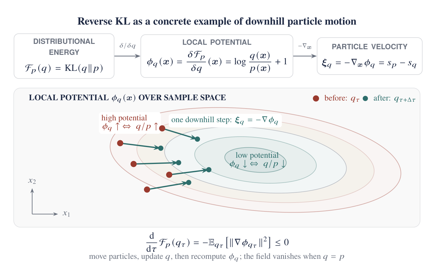
The book's LaTeX figure mapping reverse KL from a distributional energy to a local potential and particle velocity, with particles moving downhill across the potential landscape. — The original LaTeX Wasserstein-flow figure from the book. Reverse KL becomes a local potential, whose negative spatial gradient moves particles downhill; after they move, the student density and its field must be recomputed.

At equilibrium \(q=p_t\), the two terms cancel exactly:

\[ \Delta p_t-\nabla\!\cdot(p_ts_{p_t}) =\Delta p_t-\nabla\!\cdot(\nabla p_t)=0. \]

DMD averages this KL-WGF over noise levels and projects each field through the noisy generator Jacobian:

\[ \mathcal F_{\mathrm{DMD}}(\theta) =\mathbb E_t[\gamma(t)\mathrm{KL}(q_{\theta,t}\|p_t)], \] \[ \nabla_\theta\mathcal F_{\mathrm{DMD}} =-\mathbb E_{t,\mathbf z,\boldsymbol\epsilon}\!\left[ \gamma(t)\boldsymbol\xi_t(\mathbf x_t)^\top \frac{\partial\mathbf x_t}{\partial\theta}\right]. \] (11)

Using \(s_{p_t}=-\boldsymbol\epsilon_\varphi/\sigma_t\) and \(s_{q_t}=-\boldsymbol\epsilon_\psi/\sigma_t\) recovers the usual DMD teacher-minus-fake denoiser gradient. The WGF view does not replace the two-score derivation; it explains the distributional motion induced by it.

5. Drifting Models through the KDE–score connection

DMD obtains a particle direction from two denoisers. Drifting Models obtain one from nearby real and generated samples. To compare the two cleanly, we first put every quantity in the same feature space. Let \(E\) be a frozen pretrained visual encoder, let \(\mathbf x=f_\theta(\mathbf z)\) be a generated sample, and let \(\mathbf y\sim p\) be a real sample. We write

\[ \mathbf u=E(\mathbf x), \qquad \mathbf v=E(\mathbf y), \qquad \mathbf u\sim q_E, \quad \mathbf v\sim p_E. \]

Thus \(q_E\) is the distribution of generated features and \(p_E\) is the distribution of real features. Drifting constructs a direction \(\boldsymbol\xi_{\mathrm{drift}}(\mathbf u)\), freezes one small feature-space step, and regresses the generator toward it:

\[ \widetilde{\mathbf u} =\operatorname{sg}\!\left[ \mathbf u+\eta \boldsymbol\xi_{\mathrm{drift}}(\mathbf u) \right], \qquad \mathcal L_{\mathrm{drift}} =\|E(f_\theta(\mathbf z))-\widetilde{\mathbf u}\|^2. \] (12)

The encoder weights stay frozen, but gradients through \(E\) still tell the generator how to change its output. This is exactly the detached-target wrapper from Equation (7). The new question is how neighboring features determine \(\boldsymbol\xi_{\mathrm{drift}}\).

A kernel-weighted neighborhood is a score estimator

Start with the real feature distribution \(p_E\). Draw a real feature \(\mathbf v\sim p_E\) and choose a Gaussian bandwidth \(h>0\), which controls the size of the neighborhood around \(\mathbf u\). Define the unnormalized Gaussian kernel

\[ k_h(\mathbf u,\mathbf v) =\exp\!\left( -\frac{\|\mathbf u-\mathbf v\|^2}{2h^2} \right) \]

In this feature space, \(k_h\) assigns a large weight to features near \(\mathbf u\) and a small weight to distant ones. Their normalized kernel-weighted mean is

\[ M_{p_E}^h(\mathbf u) =\frac{ \mathbb E_{\mathbf v\sim p_E} [k_h(\mathbf u,\mathbf v)\mathbf v]} {\mathbb E_{\mathbf v\sim p_E} [k_h(\mathbf u,\mathbf v)]}. \]

Write the KDE density explicitly

Suppose we have \(N\) real features \(\mathbf v_1,\ldots,\mathbf v_N\sim p_E\). Place a Gaussian bump around each one and evaluate those bumps at \(\mathbf u\). Their average is

\[ \frac{C_h}{N}\sum_{i=1}^{N} k_h(\mathbf u,\mathbf v_i), \qquad C_h=(2\pi h^2)^{-d/2}. \]

where \(d\) is the feature dimension and \(C_h\) normalizes each Gaussian. In the population notation, the sample average becomes an expectation:

\[ (p_E)_h(\mathbf u) =C_h\, \mathbb E_{\mathbf v\sim p_E} [k_h(\mathbf u,\mathbf v)]. \]

Thus \((p_E)_h(\mathbf u)\) is simply a smoothed measure of how many real features lie near \(\mathbf u\).

Differentiate one kernel weight

Only the exponent depends on \(\mathbf u\). Applying the ordinary chain rule,

\[ \begin{aligned} \nabla_{\mathbf u}k_h(\mathbf u,\mathbf v) &=k_h(\mathbf u,\mathbf v) \nabla_{\mathbf u}\!\left( -\frac{\|\mathbf u-\mathbf v\|^2}{2h^2} \right)\\ &=k_h(\mathbf u,\mathbf v) \frac{\mathbf v-\mathbf u}{h^2}. \end{aligned} \]

Differentiate the log density

The Gaussian kernel lets us move the derivative inside the expectation. The constant \(C_h\) then cancels between the numerator and denominator:

\[ \begin{aligned} \nabla_{\mathbf u}\log (p_E)_h(\mathbf u) &=\frac{ \nabla_{\mathbf u}(p_E)_h(\mathbf u)} {(p_E)_h(\mathbf u)}\\ &=\frac{ C_h\mathbb E_{\mathbf v\sim p_E}[ \nabla_{\mathbf u}k_h(\mathbf u,\mathbf v)]} {C_h\mathbb E_{\mathbf v\sim p_E}[ k_h(\mathbf u,\mathbf v)]}\\ &=\frac{1}{h^2} \frac{ \mathbb E_{\mathbf v\sim p_E}[ k_h(\mathbf u,\mathbf v)(\mathbf v-\mathbf u)]} {\mathbb E_{\mathbf v\sim p_E}[ k_h(\mathbf u,\mathbf v)]}\\ &=\frac{1}{h^2}\left( \frac{ \mathbb E_{\mathbf v\sim p_E}[ k_h(\mathbf u,\mathbf v)\mathbf v]} {\mathbb E_{\mathbf v\sim p_E}[ k_h(\mathbf u,\mathbf v)]} -\mathbf u \right)\\ &=\boxed{ \frac{M_{p_E}^h(\mathbf u)-\mathbf u}{h^2}.} \end{aligned} \] (13)

The penultimate line is the key algebraic step: \(\mathbf u\) does not depend on the sampled neighbor \(\mathbf v\), so it comes out of the expectation and leaves the weighted mean \(M_{p_E}^h(\mathbf u)\). Equation (13) therefore says that the vector from \(\mathbf u\) to the local mean of nearby real features points uphill in the smoothed real density.

We now repeat exactly the same construction with generated neighbors \(\mathbf u'\sim q_E\). Their weighted mean \(M_{q_E}^h(\mathbf u)\) satisfies

\[ \nabla_{\mathbf u}\log (q_E)_h(\mathbf u) =\frac{M_{q_E}^h(\mathbf u)-\mathbf u}{h^2}. \]

So the real batch estimates the target feature score, and the generated batch estimates the model feature score. Neither estimate requires training another neural network.

Apply the same construction once to real features and once to generated features, then subtract:

\[ \begin{aligned} \boldsymbol\xi_{\mathrm{drift}}(\mathbf u) &=\bigl(M_{p_E}^h(\mathbf u)-\mathbf u\bigr) -\bigl(M_{q_E}^h(\mathbf u)-\mathbf u\bigr)\\ &=M_{p_E}^h(\mathbf u)-M_{q_E}^h(\mathbf u)\\ &=\boxed{ h^2\left[ \nabla\log (p_E)_h(\mathbf u) -\nabla\log (q_E)_h(\mathbf u) \right].} \end{aligned} \] (14)

This is the connection to score distillation. DMD estimates \(s_{p_t}-s_{q_t}\) on Gaussian-noised marginals with teacher and fake denoisers. The Gaussian KDE view of Drifting estimates the same target-score minus self-score shape on smoothed feature distributions, using real and generated neighbors instead. The real neighborhood supplies attraction; the generated neighborhood supplies the self term that keeps all particles from following the same attraction.

The KDE identity explains the connection, not every implementation detail Equation (14) is exact for the normalized Gaussian mean-shift field above. Practical Drifting Models use different affinities, joint row/column normalization, cross-weighting, and multiple feature levels. Those choices preserve the target-minus-self design, but they do not turn the production field into an exact KL or Wasserstein gradient flow automatically.

Why do we need a pretrained encoder?

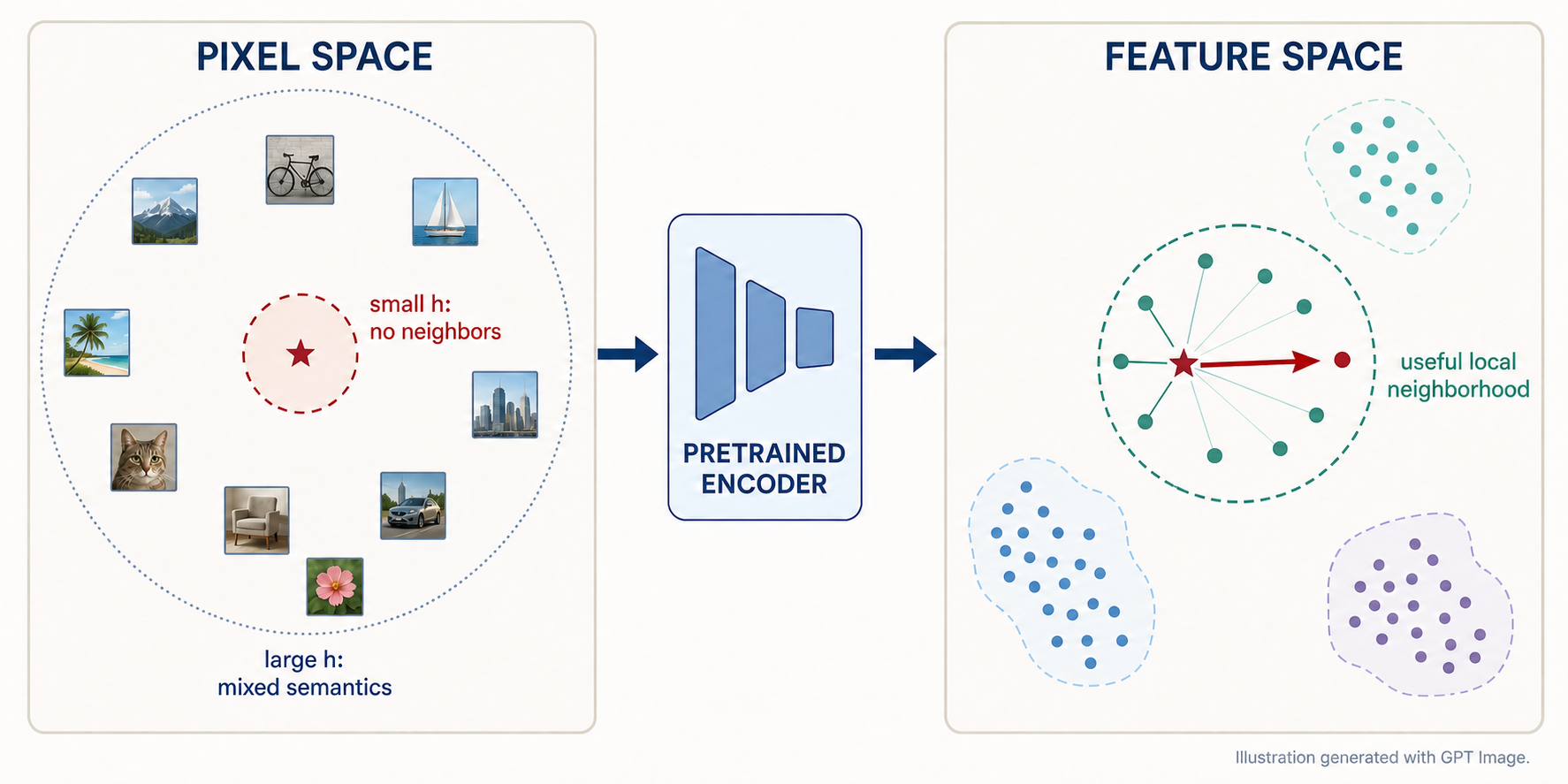
The KDE view makes its role concrete. Natural images live in an enormous pixel space but concentrate near a much thinner, lower-dimensional manifold. With only a finite batch, almost every pair of images is therefore far apart in pixel-space Euclidean distance. A small bandwidth makes nearly every kernel weight vanish; a large bandwidth prevents the weights from distinguishing genuinely local neighbors. Pixel distance is also poorly aligned with semantics: shifting an otherwise identical image by a few pixels can produce a larger distance than changing its content.

A pretrained visual encoder maps images into a space with lower effective dimension and more meaningful local geometry. There, nearby points are more likely to represent semantically similar images, so a finite batch can provide a useful local density—and therefore score—estimate. From this perspective, pretrained hidden features are not merely a perceptual-loss choice: they are what makes the neighborhood-based probability approximation plausible in the first place. Using multiple feature levels and scales supplies such neighborhoods at several levels of abstraction.

A diagram showing that Gaussian neighborhoods in high-dimensional pixel space either have no nearby samples or mix unrelated images, while a pretrained encoder creates a feature space where related samples provide a useful local direction. — Why the encoder matters from the KDE perspective. Pixel-space distances make the kernel neighborhood either empty or indiscriminate. Pretrained features create a more semantic local geometry, so nearby real samples can define a useful density and score estimate.

6. W-Flow changes how the batch interaction is normalized

W-Flow keeps the same outer training loop: encode real and generated batches, construct a feature-space direction, freeze \(\mathbf u+\eta\boldsymbol\xi(\mathbf u)\), and regress the generator toward it. The difference is the rule used to coordinate the neighbors. Drifting builds local similarity weights; W-Flow solves a globally balanced soft transport problem with Sinkhorn iterations.

Write \(\widehat q_E=\{\mathbf u_i\}\) for the current generated feature batch, \(\widehat p_E=\{\mathbf v_j\}\) for the real feature batch, and \(\widehat q'_E=\{\mathbf u'_\ell\}\) for an independent second generated batch. For a regularization strength \(\lambda>0\), let \(T^\lambda_{\widehat q_E,\widehat p_E}(\mathbf u_i)\) be the average real destination assigned to \(\mathbf u_i\) by the generated-to-real Sinkhorn plan. Define \(T^\lambda_{\widehat q_E,\widehat q'_E}(\mathbf u_i)\) analogously for self-transport. The implemented direction is

\[ \boxed{ \boldsymbol\xi_{\mathrm{W\text{-}Flow}}^\lambda(\mathbf u_i) =T^\lambda_{\widehat q_E,\widehat p_E}(\mathbf u_i) -T^\lambda_{\widehat q_E,\widehat q'_E}(\mathbf u_i).} \] (15)

The two formulas now look deliberately parallel. Drifting uses kernel-weighted local means; W-Flow uses barycentric means from transport plans whose row and column masses are balanced jointly across the batch. The independent second generated batch prevents a particle from matching itself at zero cost. Both methods then use the detached regression target in Equation (12).

At the population level, the W-Flow field is derived from the Wasserstein gradient of a debiased Sinkhorn divergence. That derivation is what makes W-Flow more than a different neighbor-weighting heuristic, but we do not need the full optimal-transport proof to understand its implementation here.

7. The comparison that survives the algebra

	DMD	Drifting Models	W-Flow
Objects being compared	Noisy marginals \(q_t\) and \(p_t\)	Generated and real feature distributions \(q_E\) and \(p_E\)	Generated and real distributions in the chosen sample or feature space
Ideal or explanatory field	\(s_{p_t}-s_{q_t}\)	Designed target-minus-self field; its Gaussian mean-shift abstraction is \(h^2[\nabla\log(p_E)_h-\nabla\log(q_E)_h]\)	Population Sinkhorn field \(T^\lambda_{q,p}-T^\lambda_{q,q}\)
Practical field estimator	Teacher and fake denoisers evaluated at generated noisy samples	Real/fake feature affinities with joint row/column normalization and cross-weighting	Generated-to-real Sinkhorn plan minus an independent two-batch self-transport plan
Explicit distributional objective	Reverse KL on noisy marginals, averaged over \(t\)	Not generally identified for the practical field	Debiased Sinkhorn divergence
Role of the highlighted identity	Exact KL-WGF direction when both scores are exact	KDE identity explains the score-distillation connection, not the full production field	OT barycentric direction; not a KDE estimator
Generator update	Field–Jacobian contraction	Detached feature-target regression	Detached sample- or feature-target regression

The useful unification is therefore not “all three are the same method.” It is a shared workflow:

\[ \boxed{ \text{choose or design a population field} \;\longrightarrow\; \text{move generated particles} \;\longrightarrow\; \text{project that motion through the generator}.} \]

DMD shows the target-score minus self-score direction using denoisers. The Gaussian KDE view of Drifting recovers the same shape from feature-space neighborhoods. W-Flow keeps the same batch-field and detached-regression pattern, but replaces local kernel weighting with globally balanced Sinkhorn plans tied to an explicit transport objective. That is the useful connection—not that all three methods are identical.

References

[1]
One-step Diffusion with Distribution Matching Distillation Tianwei Yin, Michaël Gharbi, Richard Zhang, Eli Shechtman, Fredo Durand, William T. Freeman, and Taesung Park. CVPR 2024.
[2]
Generative Modeling via Drifting Mingyang Deng, He Li, Tianhong Li, Yilun Du, and Kaiming He. arXiv:2602.04770, 2026.
[3]
One-Step Generative Modeling via Wasserstein Gradient Flows Jiaqi Han, Puheng Li, Qiushan Guo, Renyuan Xu, Stefano Ermon, and Emmanuel J. Candès. arXiv:2605.11755, 2026.
[4]
On the Wasserstein Gradient Flow Interpretation of Drifting Models Arthur Gretton, Li Kevin Wenliang, Alexandre Galashov, James Thornton, Valentin De Bortoli, and Arnaud Doucet. arXiv:2605.05118, 2026.