- Linear Attention: from an \(L\times L\) matrix to a recurrent state
- Chunkwise Linear Attention: parallelizing the recurrence
- DeltaNet: correcting an association instead of only adding to it
- Chunkwise DeltaNet: parallelizing exact delta updates
- Gated Linear Attention: forgetting old state
- Test-Time Training (TTT): from a matrix state to a learned model
- Large Chunk Test-Time Training (LaCT): learning once per large chunk
Why Linear Attention?
In Part I, we introduced FlashAttention's efficient block computation, then used the same blockwise view to understand distributed Ring Attention and sparse attention. In Part II, we turned to autoregressive inference and studied the variants and kernels that make decoding cheaper: MQA and GQA, grouped-head decoding, Flash-Decoding, Paged Attention, and MLA.
Those methods remove a great deal of wasted memory traffic, and sparse attention can skip selected query–key pairs. Dense attention, however, still compares every query with every allowed key. Training a length-\(L\) sequence therefore performs \(O(L^2)\) pairwise work, and one autoregressive decode step performs \(O(L)\) work over the accumulated prefix. The longer the context becomes, the more history we must revisit for every new token.
Here we take a different route. Instead of retaining every past key and value, Linear Attention summarizes them in a fixed-size recurrent state. Training can then use \(O(L)\) work, and recurrent decode no longer becomes more expensive as the prefix grows. Kimi K3 shows that this approach can scale to a large model: it uses Kimi Delta Attention in most layers and global Gated MLA in the remaining layers. This hybrid design substantially reduces long-context memory and decoding cost.
By the end of this article, we will be able to:
- Derive Linear Attention from ordinary attention: identify exactly why removing or factorizing softmax lets us replace the \(L\times L\) attention matrix with a fixed-size recurrent state.
- Choose the right GPU schedule: understand why recurrent decode and chunkwise training implement the same layer with different Triton kernels.
- Derive the training backward pass: follow gradients across chunk boundaries and connect the reverse recurrence to the chunkwise forward pass.
- Build DeltaNet efficiently: turn its tokenwise correction rule into a WY-style rank-one representation, solve the resulting triangular system, and reuse the chunkwise Linear Attention kernel.
- Connect TTT to Linear Attention, then move from tokenwise to chunkwise learning: derive when a TTT update is exactly Linear Attention, then see how LaCT expands the update unit from one token to an entire chunk and changes the dependency pattern inside that chunk.
1. Linear Attention: from an \(L\times L\) matrix to a recurrent state
Why softmax prevents reassociation
Stack a length-\(L\) sequence into \(Q,K\in\mathbb R^{L\times d_f}\) and \(V\in\mathbb R^{L\times d_v}\). Ignoring the causal mask for one moment, ordinary attention is
The \(L\times L\) cost comes from \(QK^\top\), which contains all \(L^2\) query–key comparisons. Let us temporarily set softmax aside and look at the remaining matrix multiplications. Without softmax between them, associativity allows us to multiply \(K^\top V\) first:
On the left, we construct an \(L\times L\) matrix and then mix values. On the right, we first compress all key–value pairs into the fixed-size matrix \(K^\top V\), then let every query read it. The work changes from quadratic in \(L\) to linear in \(L\). This change of parentheses—not recurrence by itself—is the central idea behind Linear Attention.
Why can we not do the same to ordinary attention? Because softmax sits between \(QK^\top\) and \(V\):
Once we remove softmax, the reassociation is valid, but the result is no longer ordinary attention. We will now make this unnormalized computation causal and use it as the common starting point for the recurrent and chunkwise forms.
Turn the prefix into a recurrent state
Above, \(Q,K,V\) stored tokens as rows. The summary therefore appeared as \(K^\top V\in\mathbb R^{d_f\times d_v}\), and one query read it from the left:
For the recurrent form, it is more convenient to treat \(q_t,k_t,v_t\) as column vectors and let the state map a query column directly to an output column. Transposing the equation above gives
We therefore store the transposed summary \(S_t\in\mathbb R^{d_v\times d_f}\). At position \(t\), a causal model may use only the prefix \(1{:}t\), so
The transpose is only a notation choice; the kernel does not need an extra transpose operation. We could keep \(H_t=K_{1:t}^\top V_{1:t}\) and write \(\widetilde o_t^\top=q_t^\top H_t\). We use \(S_t=H_t^\top\) because it gives the convenient value-by-key update \(v_tk_t^\top\) and the column-vector read \(S_tq_t\), which we will also use for DeltaNet and TTT.
This is the same reassociation applied to every prefix. Token \(t\) writes one outer product \(v_tk_t^\top\); later queries read the accumulated matrix. Because that write is rank one, each token changes the memory only along one key direction. We will use this rank-one structure when we derive Chunkwise DeltaNet.
For a fresh sequence, we set \(S_0=0\). During continued decode, \(S_0\) instead means the state already accumulated from the cached prefix. Expanding the recurrence makes both cases explicit:
The state has only \(d_vd_f\) numbers, regardless of context length. It acts like an associative memory: a key direction selects what a value writes, and a similar query direction retrieves it. This is the fast-weight view developed explicitly in Linear Transformers Are Secretly Fast Weight Programmers.
This unnormalized read is not softmax attention: its dot-product weights can be negative and do not have to sum to one. We treat it as a different sequence model rather than an approximation that must reproduce softmax. That is also the form used by the DeltaNet derivation below.
In the equations below, \(q_t\) and \(k_t\) mean features after any nonlinear activation and per-vector normalization. The Parallel DeltaNet parameterization we study later applies SiLU followed by \(L_2\) normalization to both. We leave those preprocessing operations out of the derivations because they do not change the state-update algebra or the execution schedule.
What becomes linear—and what does not
Here, “linear” describes how the cost grows with sequence length \(L\). The state stores \(d_vd_f\) numbers. With fixed feature widths, each token costs \(O(d_vd_f)\), so a sequence of length \(L\) costs \(O(Ld_vd_f)\). During decode, the important gain is that this state does not grow when another token arrives.
The matrix state itself can still be large. If \(d_f=d_v=d\), it contains \(d^2\) values, and doubling \(d\) roughly quadruples both the state size and the work of each update. Linear in \(L\) therefore does not mean cheap in every dimension.
Training has a different problem. Decode only needs the latest state, but backward must recover how earlier updates affected later outputs. Saving one full state after every token would cost \(O(Ld_vd_f)\) memory. The next section shows how chunkwise training saves fewer boundary states and reconstructs the remaining dependencies inside each chunk.
2. Chunkwise Linear Attention: parallelizing the recurrence
The token-by-token recurrence in Equation (1) is a natural fit for decode, where tokens arrive one at a time. During training or prefill, however, the entire sequence is already available. Processing it through Equation (1) would still make token \(t+1\) wait for token \(t\), serializing work that the GPU could otherwise run in parallel. The same recurrence also has a fully parallel form. Stack tokens as rows in \(Q,K,V\) and let \(M_L\) be the lower-triangular causal mask:
This exposes large GEMMs, but it restores \(L^2\) pairwise work. The chunkwise form interpolates between these two extremes. We use square brackets to mark chunk boundaries, not a different kind of state. With zero-indexed chunks of \(C\) tokens, \(S_{[c]}=S_{cC}\): it is the same recurrent state \(S_t\), saved immediately before chunk \(c\) begins.
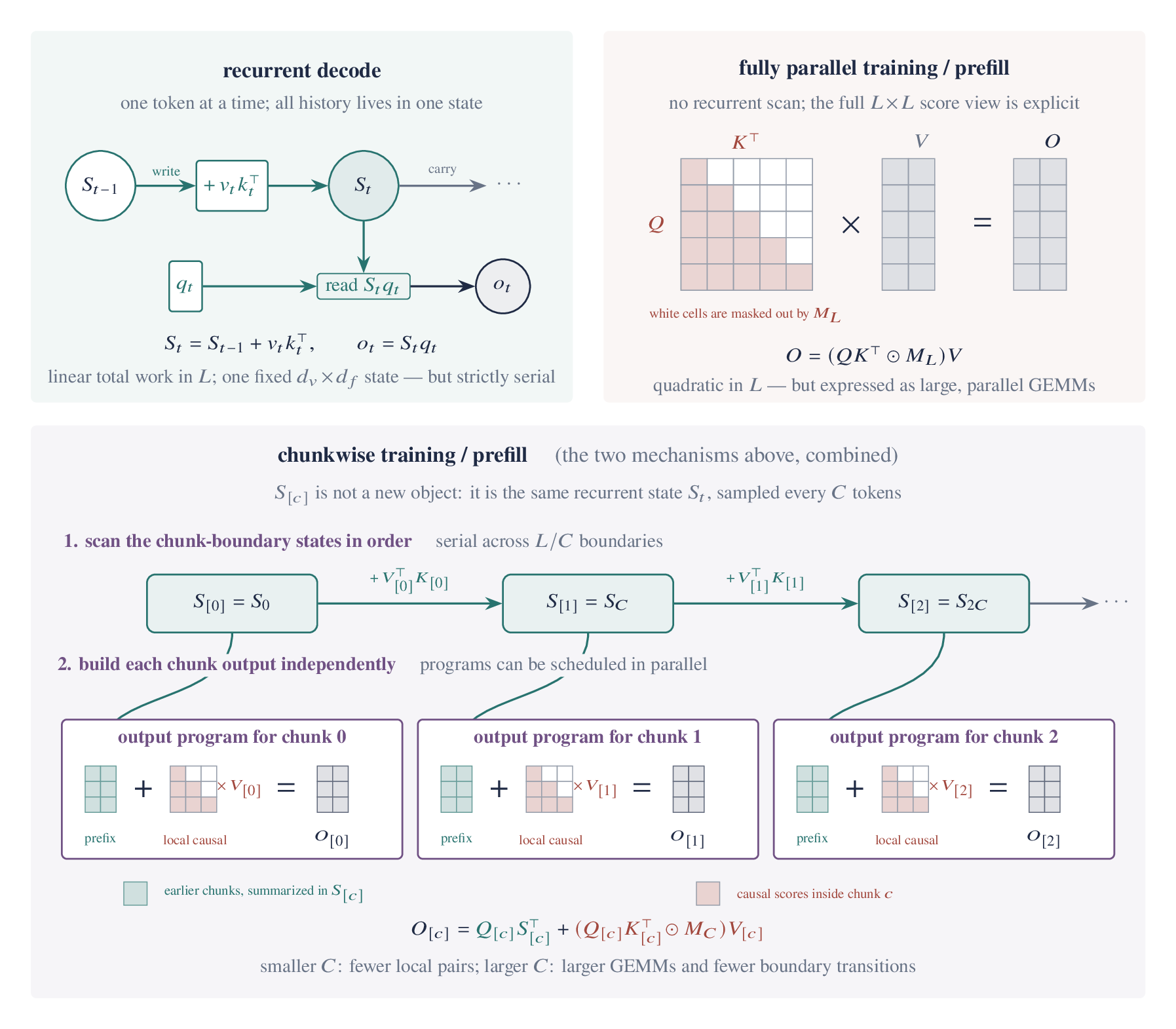
Let chunk \(c\) contain \(C\) tokens, with matrices \(Q_{[c]},K_{[c]},V_{[c]}\). For local position \(r\), we separate the incoming state from writes inside the current chunk:
The first output term reads the shared boundary state. The second is an ordinary causal attention calculation restricted to \(C\) tokens. Stacking all positions gives
Equation (4) contains both extremes. At \(C=1\), the local matrix has one element and we recover the token recurrence. At \(C=L\), there is one chunk and we recover the fully parallel quadratic form. Between them, \(C\) trades local \(C^2\) work for larger, more efficient matrix multiplications.
A common way to evaluate Equation (4) uses two kernel launches:
- Scan the boundary states. The first kernel carries one state across the chunks in sequence. Before it consumes chunk \(c\), it saves the incoming state \(S_{[c]}\); it then updates the state with \(V_{[c]}^\top K_{[c]}\). This launch is sequential along the chunk axis because \(S_{[c+1]}\) depends on \(S_{[c]}\).
- Compute the chunk outputs in parallel. After every \(S_{[c]}\) is available, the second launch assigns independent programs to different chunks. Each program loads its own \(Q_{[c]},K_{[c]},V_{[c]}\), and \(S_{[c]}\), computes both output terms in Equation (4), and writes directly to the corresponding rows of \(O\). There is no final concatenation pass.
The four matrix multiplications in Equation (4) show where the cost comes from. For one chunk:
- \(Q_{[c]}K_{[c]}^\top\) multiplies \((C\times d_f)\) by \((d_f\times C)\), costing \(O(C^2d_f)\);
- multiplying the resulting \(C\times C\) local scores by \(V_{[c]}\) costs \(O(C^2d_v)\);
- reading the incoming state with \(Q_{[c]}S_{[c]}^\top\) costs \(O(Cd_fd_v)\);
- forming the state update \(V_{[c]}^\top K_{[c]}\) costs another \(O(Cd_fd_v)\).
There are \(L/C\) chunks. Counting the leading matrix-multiplication work and omitting the same constant factor from every term, the total is
Ignoring constant factors, this is \(O(LC(d_f+d_v)+Ld_fd_v)\). This expression counts total arithmetic, not wall-clock time: the output programs can process different chunks in parallel, but parallel execution does not remove any of their multiply-accumulate operations. Only the first term grows with \(C\); the total state-reading and state-update arithmetic does not. A larger \(C\) therefore performs more local token-pair work, but exposes larger matrix multiplications and requires fewer sequential chunk transitions. A smaller \(C\) computes fewer local pairs, but creates more state hand-offs and smaller matrix multiplications.
The execution order also tells us what must be saved. In addition to the usual \(Q,K,V\) activations and output \(O\), the unnormalized path keeps one incoming state \(S_{[c]}\) per chunk, costing \(O((L/C)d_vd_f)\) elements per batch and head. It does not save \(V_{[c]}^\top K_{[c]}\) or the local attention scores. Each output program forms its \(C\times C\) score tile on chip, uses it immediately, and backward recomputes it later. Materializing all local scores would instead cost \((L/C)C^2=LC\) elements.
Triton kernels for recurrent decode and chunkwise training
To keep the implementation aligned with the main derivation, the kernels below show the complete unnormalized path. All tensors are contiguous, and \(Q\) and \(K\) already include any feature map, activation, or per-vector normalization chosen by the model.
| Parameter | Meaning |
|---|---|
Q, K | Prepared query and key features with shape \([B,H,L,D_K]\), where \(D_K=d_f\). |
V, O | Values and outputs with shape \([B,H,L,D_V]\), where \(D_V=d_v\). |
H0, HT | The recurrent state before and after the new tokens, both with shape \([B,H,D_V,D_K]\). |
H | The buffer containing one incoming state \(S_{[c]}\) per chunk, with shape \([B,H,N_C,D_V,D_K]\). |
L, NC | The number of tokens processed and the number of chunks, \(N_C=\lceil L/C\rceil\). |
DK, DV | The actual feature and value widths \(d_f,d_v\). |
BT | The number of tokens in one chunk, \(B_T=C\). |
BK, BV | The compile-time feature and value tile widths used by one Triton program. Masks remove padded lanes beyond DK and DV. |
The indexing uses one small shortcut: bh flattens batch index \(b\) and head index \(h\) into \(bH+h\). The tensors still have their ordinary \([B,H,\ldots]\) shapes; flattening only makes the launch grid and pointer arithmetic shorter. Likewise, iv selects one \(B_V\)-wide slice of the value dimension.
Recurrent decode updates the cached state and produces outputs as new tokens arrive. The kernel follows Equation (1) directly. Its launch grid is (B * H, ceil_div(DV, BV)): program_id(0) selects one flattened batch–head pair, while program_id(1) selects a block of \(B_V\) value rows from the state. A program owns those rows for the entire call, so it can loop over the new tokens without atomics. USE_H0=False starts a fresh sequence from \(S_0=0\); USE_H0=True loads a cached prefix state. In both cases, HT returns the final state for the next call.
Complete Triton kernel — recurrent decode
# Grid: (B * H, ceil_div(DV, BV))
@triton.jit
def _linear_recurrent_fwd(
    Q, K, V, O, H0, HT, L,
    DK: tl.constexpr,
    DV: tl.constexpr,
    BK: tl.constexpr,
    BV: tl.constexpr,
    USE_H0: tl.constexpr,
):
    bh = tl.program_id(0)
    iv = tl.program_id(1)

    offs_k = tl.arange(0, BK)
    offs_v = iv * BV + tl.arange(0, BV)
    mask_k = offs_k < DK
    mask_v = offs_v < DV

    state = tl.zeros([BV, BK], tl.float32)
    if USE_H0:
        p_h0 = H0 + (bh * DV + offs_v[:, None]) * DK \
                     + offs_k[None, :]
        state = tl.load(
            p_h0,
            mask=mask_v[:, None] & mask_k[None, :],
            other=0.0,
        ).to(tl.float32)

    for t in range(0, L):
        q = tl.load(Q + (bh * L + t) * DK + offs_k,
                    mask=mask_k, other=0.0)
        k = tl.load(K + (bh * L + t) * DK + offs_k,
                    mask=mask_k, other=0.0)
        v = tl.load(V + (bh * L + t) * DV + offs_v,
                    mask=mask_v, other=0.0)

        state += v[:, None] * k[None, :]
        out = tl.sum(state * q[None, :], axis=1)
        tl.store(O + (bh * L + t) * DV + offs_v,
                 out, mask=mask_v)

    p_ht = HT + (bh * DV + offs_v[:, None]) * DK \
                + offs_k[None, :]
    tl.store(
        p_ht,
        state,
        mask=mask_v[:, None] & mask_k[None, :],
    )
Chunkwise training first saves the incoming state for every chunk, then computes all chunk outputs in parallel. The boundary kernel uses the same two-dimensional grid as recurrent decode. Each program keeps one state tile in registers, walks through the chunks in order, saves \(S_{[c]}\) into H, and then advances the state with \(V_{[c]}^\top K_{[c]}\). H is therefore just the buffer of mathematical boundary states, not a second kind of state; HT is the state after the last chunk.
After that scan finishes, the output kernel launches with grid (NC, B * H, ceil_div(DV, BV)). Its first program axis selects a chunk, so different chunks now run independently. Each program loads that chunk's saved \(S_{[c]}\), forms its causal \(C\times C\) score tile, evaluates both terms of Equation (4), and stores its own slice of O.
Complete Triton kernels — chunkwise training forward
# Kernel 1: save every incoming boundary state S_[c].
# Grid: (B * H, ceil_div(DV, BV))
@triton.jit
def _linear_state_fwd(
    K, V, H, HT, L, NC,
    DK: tl.constexpr,
    DV: tl.constexpr,
    BK: tl.constexpr,
    BV: tl.constexpr,
    BT: tl.constexpr,
):
    bh = tl.program_id(0)
    iv = tl.program_id(1)

    offs_t = tl.arange(0, BT)
    offs_k = tl.arange(0, BK)
    offs_v = iv * BV + tl.arange(0, BV)
    mask_k = offs_k < DK
    mask_v = offs_v < DV

    state = tl.zeros([BV, BK], tl.float32)

    for c in range(0, NC):
        # Save S_[c] before applying chunk c's update.
        p_h = H + ((bh * NC + c) * DV + offs_v[:, None]) * DK \
                  + offs_k[None, :]
        tl.store(
            p_h,
            state,
            mask=mask_v[:, None] & mask_k[None, :],
        )

        rows = c * BT + offs_t
        valid_t = rows < L
        k = tl.load(
            K + (bh * L + rows[:, None]) * DK + offs_k[None, :],
            mask=valid_t[:, None] & mask_k[None, :],
            other=0.0,
        )
        v = tl.load(
            V + (bh * L + rows[:, None]) * DV + offs_v[None, :],
            mask=valid_t[:, None] & mask_v[None, :],
            other=0.0,
        )

        # S_[c+1] = S_[c] + V_[c]^T K_[c].
        state += tl.dot(tl.trans(v), k)

    p_ht = HT + (bh * DV + offs_v[:, None]) * DK \
                + offs_k[None, :]
    tl.store(
        p_ht,
        state,
        mask=mask_v[:, None] & mask_k[None, :],
    )


# Kernel 2: use the saved S_[c] to compute every chunk independently.
# Grid: (NC, B * H, ceil_div(DV, BV))
@triton.jit
def _linear_chunk_o_fwd(
    Q, K, V, H, O, L, NC,
    DK: tl.constexpr,
    DV: tl.constexpr,
    BK: tl.constexpr,
    BV: tl.constexpr,
    BT: tl.constexpr,
):
    c = tl.program_id(0)
    bh = tl.program_id(1)
    iv = tl.program_id(2)

    offs_t = tl.arange(0, BT)
    offs_k = tl.arange(0, BK)
    offs_v = iv * BV + tl.arange(0, BV)
    rows = c * BT + offs_t

    valid_t = rows < L
    mask_k = offs_k < DK
    mask_v = offs_v < DV

    q = tl.load(
        Q + (bh * L + rows[:, None]) * DK + offs_k[None, :],
        mask=valid_t[:, None] & mask_k[None, :],
        other=0.0,
    )
    k = tl.load(
        K + (bh * L + rows[:, None]) * DK + offs_k[None, :],
        mask=valid_t[:, None] & mask_k[None, :],
        other=0.0,
    )
    v = tl.load(
        V + (bh * L + rows[:, None]) * DV + offs_v[None, :],
        mask=valid_t[:, None] & mask_v[None, :],
        other=0.0,
    )
    h = tl.load(
        H + ((bh * NC + c) * DV + offs_v[:, None]) * DK \
          + offs_k[None, :],
        mask=mask_v[:, None] & mask_k[None, :],
        other=0.0,
    )

    # Local causal term: (Q_[c] K_[c]^T ⊙ M_C) V_[c].
    scores = tl.dot(q, tl.trans(k))
    visible = (
        valid_t[:, None]
        & valid_t[None, :]
        & (offs_t[:, None] >= offs_t[None, :])
    )
    scores = tl.where(visible, scores, 0.0)

    # Prefix term plus the local causal term from Equation (4).
    out = tl.dot(q, tl.trans(h.to(q.dtype)))
    out += tl.dot(scores.to(v.dtype), v)

    tl.store(
        O + (bh * L + rows[:, None]) * DV + offs_v[None, :],
        out,
        mask=valid_t[:, None] & mask_v[None, :],
    )
Backward: reverse the boundary scan, then differentiate each chunk
Forward split the work in two: a boundary scan produced every incoming state \(S_{[c]}\), then independent programs used those states to compute the chunk outputs. Backward mirrors that structure. The only gradient that couples neighboring chunks is the gradient of \(S_{[c]}\); once we have it, the token gradients inside different chunks can be computed independently.
For one chunk, recall the three forward operations:
As in Part I, \(dX\) denotes \(\partial\mathcal L/\partial X\), and \(dO_{[c]}\) is the upstream gradient for this chunk.
We first follow the gradient through the boundary state. Define
The state \(S_{[c]}\) reaches the loss through two paths:
- The state update copies it directly into \(S_{[c+1]}\), contributing \(G_{[c+1]}\).
- The prefix read \(Q_{[c]}S_{[c]}^\top\) contributes \(dO_{[c]}^\top Q_{[c]}\).
Adding the two contributions gives
Because \(G_{[c]}\) depends on \(G_{[c+1]}\), we must evaluate this recurrence from the final chunk toward the first. Now suppose that reverse scan has already supplied \(G_{[c+1]}\) for the current chunk. The remaining derivatives come from three familiar matrix operations.
The prefix read \(Q_{[c]}S_{[c]}^\top\) contributes
For the local interaction, we differentiate the complete expression directly:
Finally, the state update \(V_{[c]}^\top K_{[c]}\) receives \(G_{[c+1]}\) from the next boundary and contributes
Adding the contributions from these paths gives the complete gradients:
The same masked \(C\times C\) matrix appears in both \(dQ\) and \(dK\). The implementation computes it once and calls it
With this abbreviation,
The equations now expose the implementation schedule: \(G\) requires one ordered reverse scan, whereas \(E,dQ,dK,dV\) can be completed independently for every chunk.
| Launch | Grid | Equation it evaluates |
|---|---|---|
_linear_dh_bwd | (B * H, ceil_div(DV, BV)) | Reverse-scans \(G_{[c]}=G_{[c+1]}+dO_{[c]}^\top Q_{[c]}\). |
_linear_dqdk_bwd | (NC, B * H) | One program owns one chunk and finishes its \(dQ\) and \(dK\) rows. |
_linear_dv_bwd | (NC, B * H, ceil_div(DV, BV)) | One program owns one value tile of a chunk and finishes \(dV\). |
Launch 1 reverse-scans the boundary-state gradient. One program starts with zero after the final chunk, walks right to left, and saves \(G_{[c+1]}\) into DH_NEXT before adding the current chunk's \(dO_{[c]}^\top Q_{[c]}\). Here DH_NEXT has shape \([B,H,N_C,D_V,D_K]\).
Complete Triton kernel — reverse-scan the boundary-state gradient
# Grid: (B * H, ceil_div(DV, BV))
@triton.jit
def _linear_dh_bwd(Q, DO, DH_NEXT, L, NC,
                   DK: tl.constexpr, DV: tl.constexpr,
                   BK: tl.constexpr, BV: tl.constexpr,
                   BT: tl.constexpr):
    # One program owns the same state tile as the forward scan.
    bh = tl.program_id(0)
    iv = tl.program_id(1)
    offs_t = tl.arange(0, BT)
    offs_k = tl.arange(0, BK)
    offs_v = iv * BV + tl.arange(0, BV)
    mask_k = offs_k < DK
    mask_v = offs_v < DV
    dh = tl.zeros([BV, BK], tl.float32)

    for step in range(0, NC):
        c = NC - 1 - step
        p_dh = DH_NEXT + ((bh * NC + c) * DV
                 + offs_v[:, None]) * DK + offs_k[None, :]
        tl.store(p_dh, dh, mask=mask_v[:, None] & mask_k[None, :])

        rows = c * BT + offs_t
        valid_t = rows < L
        q = tl.load(Q + (bh * L + rows[:, None]) * DK
                    + offs_k[None, :],
                    mask=valid_t[:, None] & mask_k[None, :],
                    other=0.0)
        do = tl.load(DO + (bh * L + rows[:, None]) * DV
                     + offs_v[None, :],
                     mask=valid_t[:, None] & mask_v[None, :],
                     other=0.0)
        dh += tl.dot(tl.trans(do), q)
Launch 2 computes \(dQ\) and \(dK\) independently for every chunk. The kernel first accumulates contributions across the value dimension. The variables h and dh are the saved \(S_{[c]}\) and \(G_{[c+1]}\). The local \(C\times C\) variable e is the masked score gradient \(E_{[c]}\); it remains on chip and is discarded after the chunk.
Complete Triton kernel — compute dQ and dK
# Grid: (NC, B * H)
@triton.jit
def _linear_dqdk_bwd(
    Q,
    K,
    V,
    DO,
    H,
    DH_NEXT,
    DQ,
    DK_OUT,
    L,
    NC,
    DK: tl.constexpr,
    DV: tl.constexpr,
    BK: tl.constexpr,
    BV: tl.constexpr,
    BT: tl.constexpr,
):
    c = tl.program_id(0)
    bh = tl.program_id(1)
    offs_t = tl.arange(0, BT)
    offs_k = tl.arange(0, BK)
    rows = c * BT + offs_t
    valid_t = rows < L
    mask_k = offs_k < DK

    q = tl.load(
        Q + (bh * L + rows[:, None]) * DK + offs_k[None, :],
        mask=valid_t[:, None] & mask_k[None, :],
        other=0.0,
    )
    k = tl.load(
        K + (bh * L + rows[:, None]) * DK + offs_k[None, :],
        mask=valid_t[:, None] & mask_k[None, :],
        other=0.0,
    )
    dq = tl.zeros([BT, BK], tl.float32)
    dk = tl.zeros([BT, BK], tl.float32)
    e = tl.zeros([BT, BT], tl.float32)

    for start_v in range(0, DV, BV):
        offs_v = start_v + tl.arange(0, BV)
        mask_v = offs_v < DV
        v = tl.load(
            V + (bh * L + rows[:, None]) * DV + offs_v[None, :],
            mask=valid_t[:, None] & mask_v[None, :],
            other=0.0,
        )
        do = tl.load(
            DO + (bh * L + rows[:, None]) * DV + offs_v[None, :],
            mask=valid_t[:, None] & mask_v[None, :],
            other=0.0,
        )
        h = tl.load(
            H + ((bh * NC + c) * DV + offs_v[:, None]) * DK
              + offs_k[None, :],
            mask=mask_v[:, None] & mask_k[None, :],
            other=0.0,
        )
        dh = tl.load(
            DH_NEXT + ((bh * NC + c) * DV + offs_v[:, None]) * DK
                    + offs_k[None, :],
            mask=mask_v[:, None] & mask_k[None, :],
            other=0.0,
        )

        dq += tl.dot(do, h.to(do.dtype))
        e += tl.dot(do, tl.trans(v))
        dk += tl.dot(v, dh.to(v.dtype))

    causal = offs_t[:, None] >= offs_t[None, :]
    visible = valid_t[:, None] & valid_t[None, :] & causal
    e = tl.where(visible, e, 0.0)
    dq += tl.dot(e.to(k.dtype), k)
    dk += tl.dot(tl.trans(e.to(q.dtype)), q)

    tl.store(
        DQ + (bh * L + rows[:, None]) * DK + offs_k[None, :],
        dq,
        mask=valid_t[:, None] & mask_k[None, :],
    )
    tl.store(
        DK_OUT + (bh * L + rows[:, None]) * DK + offs_k[None, :],
        dk,
        mask=valid_t[:, None] & mask_k[None, :],
    )
Launch 3 computes \(dV\). It reconstructs the local causal scores and combines two paths: the local output contributes \(\left(M_C\odot Q_{[c]}K_{[c]}^\top\right)^\top dO_{[c]}\), while the state update contributes \(K_{[c]}G_{[c+1]}^\top\). Splitting the value dimension across programs is safe because each program writes disjoint columns of \(dV\).
Complete Triton kernel — compute dV
# Grid: (NC, B * H, ceil_div(DV, BV))
@triton.jit
def _linear_dv_bwd(
    Q,
    K,
    DO,
    DH_NEXT,
    DV_OUT,
    L,
    NC,
    DK: tl.constexpr,
    DV: tl.constexpr,
    BK: tl.constexpr,
    BV: tl.constexpr,
    BT: tl.constexpr,
):
    c = tl.program_id(0)
    bh = tl.program_id(1)
    iv = tl.program_id(2)
    offs_t = tl.arange(0, BT)
    offs_k = tl.arange(0, BK)
    offs_v = iv * BV + tl.arange(0, BV)
    rows = c * BT + offs_t
    valid_t = rows < L
    mask_k = offs_k < DK
    mask_v = offs_v < DV

    q = tl.load(
        Q + (bh * L + rows[:, None]) * DK + offs_k[None, :],
        mask=valid_t[:, None] & mask_k[None, :],
        other=0.0,
    )
    k = tl.load(
        K + (bh * L + rows[:, None]) * DK + offs_k[None, :],
        mask=valid_t[:, None] & mask_k[None, :],
        other=0.0,
    )
    do = tl.load(
        DO + (bh * L + rows[:, None]) * DV + offs_v[None, :],
        mask=valid_t[:, None] & mask_v[None, :],
        other=0.0,
    )
    dh = tl.load(
        DH_NEXT + ((bh * NC + c) * DV + offs_v[:, None]) * DK
                + offs_k[None, :],
        mask=mask_v[:, None] & mask_k[None, :],
        other=0.0,
    )

    scores = tl.dot(q, tl.trans(k))
    visible = (
        valid_t[:, None]
        & valid_t[None, :]
        & (offs_t[:, None] >= offs_t[None, :])
    )
    scores = tl.where(visible, scores, 0.0)

    dv = tl.dot(tl.trans(scores.to(do.dtype)), do)
    dv += tl.dot(k, tl.trans(dh.to(k.dtype)))
    tl.store(
        DV_OUT + (bh * L + rows[:, None]) * DV + offs_v[None, :],
        dv,
        mask=valid_t[:, None] & mask_v[None, :],
    )
The reverse scan must finish before the independent \(dQ,dK,dV\) kernels can read DH_NEXT. The wrapper therefore launches the three kernels in exactly this order:
Complete Python launcher — unnormalized Linear Attention backward
def linear_chunk_backward(q, k, v, h, do, chunk_size):
    B, H, L, DK, DV = _check_qkv(q, k, v)
    BT = chunk_size
    NC = triton.cdiv(L, BT)
    BK, BV = _blocks(DK, DV)
    bh = B * H
    nv = triton.cdiv(DV, BV)

    do = do.contiguous()
    dh_next = torch.empty_like(h)
    dq = torch.empty_like(q)
    dk = torch.empty_like(k)
    dv = torch.empty_like(v)

    # 1. Reverse-scan G_[c+1].
    _linear_dh_bwd[(bh, nv)](
        q,
        do,
        dh_next,
        L,
        NC,
        DK=DK,
        DV=DV,
        BK=BK,
        BV=BV,
        BT=BT,
        num_warps=4,
    )

    # 2. Every chunk independently finishes dQ and dK.
    _linear_dqdk_bwd[(NC, bh)](
        q,
        k,
        v,
        do,
        h,
        dh_next,
        dq,
        dk,
        L,
        NC,
        DK=DK,
        DV=DV,
        BK=BK,
        BV=BV,
        BT=BT,
        num_warps=4,
    )

    # 3. Value tiles independently finish dV.
    _linear_dv_bwd[(NC, bh, nv)](
        q,
        k,
        do,
        dh_next,
        dv,
        L,
        NC,
        DK=DK,
        DV=DV,
        BK=BK,
        BV=BV,
        BT=BT,
        num_warps=4,
    )
    return dq, dk, dv
Open the complete Triton implementation and PyTorch reference checks
3. DeltaNet: correcting an association instead of only adding to it
Before comparing the two update rules, we should make the roles of \(k\), \(v\), and \(q\) explicit. A key–value pair says that when the state is addressed by \(k_t\), we want it to return \(v_t\):
The key is the address and the value is the content stored there. The query does not define this association; it searches the completed map. For the additive state,
Therefore, when \(q\) is close to \(k_j\), the match score \(k_j^\top q\) is large and the corresponding \(v_j\) contributes strongly to the output. We first store the relation \(k_j\mapsto v_j\); similarity between \(q\) and \(k_j\) is what later lets us retrieve it.
The problem with the additive update is that it never checks whether the mapping already satisfies \(S_{t-1}k_t\approx v_t\). It simply adds another outer product. For a unit-norm key, let \(\hat v_t=S_{t-1}k_t\) be the value currently associated with \(k_t\). Then
The first write into an empty state works, but a repeated write adds the value again. If the association has changed, a future query close to \(k_t\) retrieves a mixture of the old and new values. Because a fixed-dimensional state must compress many associations, such overlapping key directions cannot always be avoided.
DeltaNet adds the missing operation: read before writing. It asks what the state currently associates with \(k_t\), then writes only the error:
If the memory already returns the desired value, \(e_t=0\). If it returns an outdated value, \(e_t\) is exactly the correction needed to move that association toward \(v_t\). The model chooses the write strength \(\beta_t=\sigma(W_\beta x_t)\in(0,1)\), giving the update
The first line is the read–correct–write view. The second is the equivalent erase–write view that we will use in the chunkwise derivation. For the same unit-norm key,
When \(\beta_t=1\), the mapping at \(k_t\) is corrected to \(S_tk_t=v_t\) exactly; a smaller \(\beta_t\) interpolates between the old and new values. A later query \(q\) reads this corrected map through
If \(q\) is close to \(k_t\), the corrected association receives a large weight and pulls the output toward the updated \(v_t\); an orthogonal query receives none of that correction. Equivalently, this residual write is one gradient step on \(\frac12\lVert Sk_t-v_t\rVert_2^2\). DeltaNet does not remove all interference from a finite state, but it gives that state a direct way to correct an existing key–value relation. This is especially valuable for associative recall, where delta-rule models have been found more effective than purely additive variants.
The price of this stronger update is a new dependency: \(e_t=v_t-S_{t-1}k_t\) cannot be known until the previous state exists. The next section shows how we preserve this tokenwise rule while exposing parallel work inside each chunk.
4. Chunkwise DeltaNet: parallelizing exact delta updates
The tokenwise Delta rule is already a good schedule for decode: one new token arrives, reads the latest state, and updates it once. Training and prefill are different because every token in the sequence is already available. Running the same loop from left to right would make each token wait for the preceding state and leave us with almost no parallelism along the sequence dimension.
Section 2 avoided that problem for additive Linear Attention. Every write \(v_rk_r^\top\) was known before the chunk began, so we could compute the chunk's local interactions with matrix multiplications and pass only one boundary state to the next chunk. DeltaNet cannot use that formula directly: its effective write \(\beta_r(v_r-S^{r-1}k_r)k_r^\top\) is unknown until all earlier writes in the chunk have produced \(S^{r-1}\).
Our goal is therefore precise. Given the incoming state \(S_{[c]}\) and all \(K,V,\beta\) values in a chunk, we want every token output and the final state \(S_{[c+1]}\). The result must exactly match the tokenwise recurrence, but we do not want to save one full \(d_v\times d_f\) state per token or execute the entire chunk as a serial loop.
First attempt: compose the token updates with a parallel scan
To see what can be parallelized, rewrite Equation (5) as an affine state transition:
Here \(M_r\) is the DeltaNet transition matrix; it is unrelated to the causal mask \(M_C\) used earlier. Expanding the first two positions makes the dependency visible:
Now the pattern is visible. The incoming state is multiplied by every transition. A write \(X_i\) is multiplied only by the transitions that come after it. After \(r\) positions,
The products follow token order, and an empty product is the identity. Thus \(P_r\) describes how the incoming state passes through the first \(r\) transitions, while \(H_r\) collects the writes created along the way.
Because affine maps compose associatively, a prefix scan could reduce the sequential depth from \(C\) to \(O(\log C)\). But if we represent these maps as dense \(d\times d\) matrices, every combine still costs \(O(d^3)\) and creates another dense intermediate. This loses the \(O(d^2)\) rank-one structure of the original Delta update. Directly computing these transformations with dense matrix multiplication is therefore impractical.
The rank-one structure gives us the WY representation
The escape hatch is that \(M_r\) is not a generic dense matrix. It is the identity minus one vector outer product. Multiplying just two such transitions shows the structure we can preserve:
The product may be numerically dense, but we never need to materialize it as a dense matrix. We keep the original right vectors \(k_i^\top\) and update only their left vectors \(w_i\). Computing the cross term requires the scalar similarity \(k_1^\top k_2\), not a \(d\times d\) by \(d\times d\) multiplication.
According to the WY representation introduced by Bischof and Van Loan, as applied to DeltaNet by Songlin Yang, the two terms in Equation (6) can be written as
The base case follows directly from the definitions:
Thus \(w_1=\beta_1k_1\) and \(u_1=\beta_1v_1\). For the induction step, suppose the representation holds through position \(r-1\). Start with the transition product \(P_r=P_{r-1}M_r\) and multiply out every term:
The cross terms all share the new right vector \(k_r^\top\), so they can be absorbed into one new left vector \(w_r\). The write accumulator follows the same pattern:
Both forms are therefore preserved when we append position \(r\), which completes the induction. The underbraced coefficients give the constructive recurrences
The two recurrences have the same coefficients because both paths pass through the same erase matrices. The \(w_r\) vectors describe how those erases transform the incoming state; the \(u_r\) vectors describe how they transform the values written inside the chunk. We have replaced dense matrix products with key similarities and vector updates, and the large \(d_v\times d_f\) state no longer appears inside the chunk-local recurrence.
One sequential dependency remains: row \(r\) uses the earlier \(u_i\) and \(w_i\). Fortunately, every such dependency is weighted only by the scalar key similarity \(k_i^\top k_r\). Collecting all of those scalars in \(KK^\top\) turns the vector recurrences into one triangular system.
From vector recurrences to one triangular solve
Stack \(w_r^\top,k_r^\top,u_r^\top,v_r^\top\) as rows of \(W,K,U,V\), and let \(B=\operatorname{diag}(\beta)\). Transpose Equation (7), expand the parentheses, and move the earlier-row terms to the left:
These coefficients define a \(C\times C\) matrix. Let
The matrix is lower triangular because row \(r\) depends only on rows \(i\le r\). Now row \(r\) of \(AW\) is exactly the left-hand side of the \(w\) equation above, while row \(r\) of \(BK\) is its right-hand side. The \(u\) recurrence uses the same coefficients, so it shares the same matrix \(A\):
We have moved the hard dimension from the feature width \(d\) to the chunk length \(C\). Forming \(KK^\top\) costs \(O(C^2d_f)\); applying the triangular solve to the key and value right-hand sides costs \(O(C^2(d_f+d_v))\). Solving or assembling the small \(C\times C\) system itself can cost \(O(C^3)\), but there is no longer a \(d^3\) term. In practice \(C\) is a controlled tile size such as 16, 32, or 64, and these operations can be expressed as GPU-friendly matrix multiplications.
Example · A three-token triangular system
Forward substitution first solves row \(1\). Row \(2\) subtracts the influence of row \(1\); row \(3\) subtracts rows \(1\) and \(2\). This is exactly the dependency order in Equation (7), but all feature/value columns are solved together. The matrix is triangular because a causal token may depend on earlier tokens, never later ones.
With two tokens, we can check the recurrence directly:
This is exactly the \(r=2\) recurrence in Equation (7); replacing \(w,k\) by \(u,v\) gives the value-path equation. The triangular solve is therefore not a new approximation—it evaluates all of those causal row recurrences in one batched linear-algebra operation.
Build a \(64\times64\) inverse from \(16\times16\) blocks
To turn the triangular solve into GPU work, we write \(T=A^{-1}\), so that \(W=T(BK)\) and \(U=T(BV)\). The number 16 is not required by the mathematics; it is the base tile size chosen by this Triton implementation. For each diagonal block \(A_{16}^{[j]}\), we solve
Because \(A_{16}^{[j]}\) is unit lower triangular, we can solve this equation from its first row to its last row; this row-by-row procedure is forward substitution. The four diagonal blocks of a \(64\times64\) matrix do not overlap, so four Triton programs can solve them independently.
The full decomposition has two levels, not one. First split \(A_{64}\) into two \(32\times32\) diagonal blocks; then split each of those into two \(16\times16\) diagonal blocks:
Here the \(G\) blocks are the off-diagonal parts that connect the later rows to the earlier rows. Once we have reached the four \(16\times16\) diagonal blocks, we reverse the process and assemble their inverses. Every merge uses the same block identity:
The two smaller inverses, \(T_{11}\) and \(T_{22}\), remain on the diagonal. The upper-right block stays zero, so the merge only computes the new lower-left block \(-T_{22}A_{21}T_{11}\). Applied recursively, the construction is
_delta_solve_16_fwdproduces the four \(T_{16}^{[j]}\) blocks in parallel._delta_merge_32_fwdmerges neighboring pairs, producing \(T_{32}^{[0]}\) and \(T_{32}^{[1]}\)._delta_merge_64_fwdkeeps those two results on the diagonal and computes the final \(32\times32\) lower-left block, producing \(T_{64}\).
The base solve contains a short 16-row dependency, while the 32- and 64-row merges are matrix multiplications.
Recover ordinary chunkwise Linear Attention
Substitute the compact forms into \(S^r=S_{[c]}P_r+H_r\):
Define the effective value rows for the whole chunk:
Substituting Equation (9), DeltaNet has exactly the same chunk formula as Equation (4), with \(V\) replaced by \(\bar V\):
Equation (5) defined a genuinely token-by-token update. Equations (6)–(8) solved all of its within-chunk dependencies using rank-one factors and a triangular system. Equation (9) packaged the result as corrected values. Equation (10) then reused an ordinary chunkwise Linear Attention kernel. The schedule changed; the per-token Delta rule did not.
The Triton preparation follows the algebra in three stages. First we form the strict lower triangle of \(BKK^\top\) once. Next we solve 16-row diagonal blocks and combine them into the requested chunk size. Finally, ordinary tl.dot operations apply \(T\) to \(BK\) and \(BV\). This keeps the small unavoidable triangular dependency separate from the large feature and value matrix products.
| Buffer | Shape | Meaning |
|---|---|---|
BETA | \([B,H,L]\) | The learned write strength \(\beta_t\) for every token. |
A | \([B,H,N_C,B_T,B_T]\) | The strict lower triangle of \(\beta KK^\top\). Its diagonal identity is implicit. |
AINV | \([B,H,N_C,B_T,B_T]\) | The inverse of the full unit-lower-triangular system. Since the code buffer A omits the identity diagonal, this is \(T=(I+\texttt{A})^{-1}\). |
W | \([B,H,L,D_K]\) | The key-side compact-WY factor \(T(\beta K)\). |
U | \([B,H,L,D_V]\) | The value-side factor \(T(\beta V)\). |
VBAR | \([B,H,L,D_V]\) | The corrected values \(\bar V=U-WS_{[c]}^\top\). |
H | \([B,H,N_C,D_V,D_K]\) | The incoming state \(S_{[c]}\) saved for every chunk. |
The Python launcher makes the execution order explicit:
_delta_kkt_fwdforms the strict lower triangle._delta_solve_16_fwdsolves every \(16\times16\) diagonal block._delta_merge_32_fwdand, when needed,_delta_merge_64_fwdassemble the requested 32- or 64-token solve._delta_w_fwdand_delta_u_fwdapply the solved matrix to the two right-hand sides._delta_state_fwdconstructs \(\bar V\) while scanning the chunk-boundary state.- The already defined
_linear_chunk_o_fwdevaluates Equation (10) with \(V\) replaced by \(\bar V\).
Complete Triton kernels — DeltaNet chunk forward
# Grid: (NC, B * H)
@triton.jit
def _delta_kkt_fwd(
    K,
    BETA,
    A,
    L,
    NC,
    DK: tl.constexpr,
    BK: tl.constexpr,
    BT: tl.constexpr,
):
    """Form the one shared strictly lower-triangular beta K K^T matrix."""
    c = tl.program_id(0)
    bh = tl.program_id(1)
    offs_t = tl.arange(0, BT)
    offs_k = tl.arange(0, BK)
    rows = c * BT + offs_t
    valid_t = rows < L
    k = tl.load(
        K + (bh * L + rows[:, None]) * DK + offs_k[None, :],
        mask=valid_t[:, None] & (offs_k[None, :] < DK),
        other=0.0,
    )
    beta = tl.load(BETA + bh * L + rows, mask=valid_t, other=0.0).to(tl.float32)
    a = tl.dot(k, tl.trans(k)) * beta[:, None]
    lower = offs_t[:, None] > offs_t[None, :]
    a = tl.where(valid_t[:, None] & valid_t[None, :] & lower, a, 0.0)

    tl.store(
        A
        + ((bh * NC + c) * BT + offs_t[:, None]) * BT
        + offs_t[None, :],
        a,
    )


# Grid: (NC, B * H, BT // 16)
@triton.jit
def _delta_solve_16_fwd(
    A,
    AINV,
    NC,
    BT: tl.constexpr,
):
    """Invert one 16x16 diagonal block of I + A by forward substitution."""
    c = tl.program_id(0)
    bh = tl.program_id(1)
    block = tl.program_id(2)
    offs = tl.arange(0, 16)
    block_offs = block * 16 + offs
    p_a = (
        A
        + ((bh * NC + c) * BT + block_offs[:, None]) * BT
        + block_offs[None, :]
    )
    a = tl.load(p_a).to(tl.float32)
    inverse = tl.zeros([16, 16], tl.float32)

    # A stores only the strict lower triangle. Each new inverse row depends
    # on the rows already completed above it; all 16 columns advance together.
    for r in tl.static_range(0, 16):
        is_r = offs == r
        a_r = tl.sum(tl.where(is_r[:, None], a, 0.0), axis=0)
        inverse_r = is_r.to(tl.float32) - tl.sum(a_r[:, None] * inverse, axis=0)
        inverse = tl.where(is_r[:, None], inverse_r[None, :], inverse)

    tl.store(
        AINV
        + ((bh * NC + c) * BT + block_offs[:, None]) * BT
        + block_offs[None, :],
        inverse,
    )


# Grid: (NC, B * H, BT // 32)
@triton.jit
def _delta_merge_32_fwd(
    A,
    AINV,
    NC,
    BT: tl.constexpr,
):
    """Merge two inverted 16x16 blocks into one 32x32 inverse."""
    c = tl.program_id(0)
    bh = tl.program_id(1)
    pair = tl.program_id(2)
    offs = tl.arange(0, 16)
    base = pair * 32
    top = base + offs
    bottom = base + 16 + offs
    chunk = (bh * NC + c) * BT * BT

    ai11 = tl.load(AINV + chunk + top[:, None] * BT + top[None, :]).to(tl.float32)
    ai22 = tl.load(AINV + chunk + bottom[:, None] * BT + bottom[None, :]).to(tl.float32)
    a21 = tl.load(A + chunk + bottom[:, None] * BT + top[None, :])
    left = tl.dot(ai22, a21, input_precision="ieee")
    ai21 = -tl.dot(left, ai11, input_precision="ieee")
    tl.store(AINV + chunk + bottom[:, None] * BT + top[None, :], ai21)


# Grid: (NC, B * H)
@triton.jit
def _delta_merge_64_fwd(
    A,
    AINV,
    NC,
    BT: tl.constexpr,
):
    """Merge the two 32x32 diagonal inverses when BT is 64."""
    c = tl.program_id(0)
    bh = tl.program_id(1)
    offs = tl.arange(0, 32)
    chunk = (bh * NC + c) * BT * BT
    lower = offs[:, None] >= offs[None, :]

    ai11 = tl.load(AINV + chunk + offs[:, None] * BT + offs[None, :]).to(tl.float32)
    ai11 = tl.where(lower, ai11, 0.0)
    ai22 = tl.load(
        AINV + chunk + (32 + offs[:, None]) * BT + 32 + offs[None, :]
    ).to(tl.float32)
    ai22 = tl.where(lower, ai22, 0.0)
    a21 = tl.load(A + chunk + (32 + offs[:, None]) * BT + offs[None, :])
    left = tl.dot(ai22, a21, input_precision="ieee")
    ai21 = -tl.dot(left, ai11, input_precision="ieee")
    tl.store(
        AINV + chunk + (32 + offs[:, None]) * BT + offs[None, :],
        ai21,
    )


# Grid: (NC, B * H)
@triton.jit
def _delta_w_fwd(
    AINV,
    K,
    BETA,
    W,
    L,
    NC,
    DK: tl.constexpr,
    BK: tl.constexpr,
    BT: tl.constexpr,
):
    """Apply the solved triangular system to beta K with one tl.dot."""
    c = tl.program_id(0)
    bh = tl.program_id(1)
    offs_t = tl.arange(0, BT)
    offs_k = tl.arange(0, BK)
    rows = c * BT + offs_t
    valid_t = rows < L
    lower = offs_t[:, None] >= offs_t[None, :]
    ainv = tl.load(
        AINV
        + ((bh * NC + c) * BT + offs_t[:, None]) * BT
        + offs_t[None, :]
    )
    ainv = tl.where(lower, ainv, 0.0)
    k = tl.load(
        K + (bh * L + rows[:, None]) * DK + offs_k[None, :],
        mask=valid_t[:, None] & (offs_k[None, :] < DK),
        other=0.0,
    )
    beta = tl.load(BETA + bh * L + rows, mask=valid_t, other=0.0).to(tl.float32)
    rhs = (k * beta[:, None]).to(K.dtype.element_ty)
    w = tl.dot(ainv, rhs)

    tl.store(
        W + (bh * L + rows[:, None]) * DK + offs_k[None, :],
        w,
        mask=valid_t[:, None] & (offs_k[None, :] < DK),
    )


# Grid: (NC, B * H, ceil_div(DV, BV))
@triton.jit
def _delta_u_fwd(
    AINV,
    V,
    BETA,
    U,
    L,
    NC,
    DV: tl.constexpr,
    BV: tl.constexpr,
    BT: tl.constexpr,
):
    """Apply the same solved triangular system to each beta V tile."""
    c = tl.program_id(0)
    bh = tl.program_id(1)
    iv = tl.program_id(2)
    offs_t = tl.arange(0, BT)
    offs_v = iv * BV + tl.arange(0, BV)
    rows = c * BT + offs_t
    valid_t = rows < L
    lower = offs_t[:, None] >= offs_t[None, :]
    ainv = tl.load(
        AINV
        + ((bh * NC + c) * BT + offs_t[:, None]) * BT
        + offs_t[None, :]
    )
    ainv = tl.where(lower, ainv, 0.0)
    v = tl.load(
        V + (bh * L + rows[:, None]) * DV + offs_v[None, :],
        mask=valid_t[:, None] & (offs_v[None, :] < DV),
        other=0.0,
    )
    beta = tl.load(BETA + bh * L + rows, mask=valid_t, other=0.0).to(tl.float32)
    rhs = (v * beta[:, None]).to(V.dtype.element_ty)
    u = tl.dot(ainv, rhs)

    tl.store(
        U + (bh * L + rows[:, None]) * DV + offs_v[None, :],
        u,
        mask=valid_t[:, None] & (offs_v[None, :] < DV),
    )


# Grid: (B * H, ceil_div(DV, BV))
@triton.jit
def _delta_state_fwd(
    K,
    W,
    U,
    VBAR,
    H,
    L,
    NC,
    DK: tl.constexpr,
    DV: tl.constexpr,
    BK: tl.constexpr,
    BV: tl.constexpr,
    BT: tl.constexpr,
):
    """Construct corrected values, then scan the ordinary additive state."""
    bh = tl.program_id(0)
    iv = tl.program_id(1)
    offs_t = tl.arange(0, BT)
    offs_k = tl.arange(0, BK)
    offs_v = iv * BV + tl.arange(0, BV)
    mask_k = offs_k < DK
    mask_v = offs_v < DV
    state = tl.zeros([BV, BK], tl.float32)

    for c in range(0, NC):
        tl.store(
            H + ((bh * NC + c) * DV + offs_v[:, None]) * DK + offs_k[None, :],
            state,
            mask=mask_v[:, None] & mask_k[None, :],
        )
        rows = c * BT + offs_t
        valid_t = rows < L
        k = tl.load(
            K + (bh * L + rows[:, None]) * DK + offs_k[None, :],
            mask=valid_t[:, None] & mask_k[None, :],
            other=0.0,
        )
        w = tl.load(
            W + (bh * L + rows[:, None]) * DK + offs_k[None, :],
            mask=valid_t[:, None] & mask_k[None, :],
            other=0.0,
        )
        u = tl.load(
            U + (bh * L + rows[:, None]) * DV + offs_v[None, :],
            mask=valid_t[:, None] & mask_v[None, :],
            other=0.0,
        )
        vbar = u.to(tl.float32) - tl.dot(w, tl.trans(state.to(w.dtype)))
        tl.store(
            VBAR + (bh * L + rows[:, None]) * DV + offs_v[None, :],
            vbar,
            mask=valid_t[:, None] & mask_v[None, :],
        )
        state += tl.dot(tl.trans(vbar.to(k.dtype)), k)
The last Delta-specific kernel owns one value tile of \(S\). It walks over chunks, saves \(S_{[c]}\), constructs \(\bar V\) from Equation (9), and immediately applies the additive update \(S_{[c+1]}=S_{[c]}+\bar V_{[c]}^\top K_{[c]}\). The ordinary chunk-output kernel from Section 2 then consumes \(Q,K,\bar V\), so we reuse that complete implementation rather than duplicate it.
Complete Python launcher — DeltaNet chunk forward
def delta_chunk(
    q: torch.Tensor,
    k: torch.Tensor,
    v: torch.Tensor,
    beta: torch.Tensor,
    *,
    chunk_size: int = 32,
) -> torch.Tensor:
    """Exact chunked DeltaNet forward using a Triton compact-WY preparation."""
    B, H, L, DK, DV = _check_qkv(q, k, v)
    if (
        beta.shape != (B, H, L)
        or not beta.is_cuda
        or not beta.is_contiguous()
        or beta.dtype != q.dtype
    ):
        raise ValueError("beta must be contiguous [B,H,L] with the same CUDA dtype as q")
    if chunk_size not in (16, 32, 64):
        raise ValueError("chunk_size must be 16, 32, or 64")
    NC = triton.cdiv(L, chunk_size)
    BK, BV = _blocks(DK, DV)
    bh, nv = B * H, triton.cdiv(DV, BV)
    a = torch.empty((B, H, NC, chunk_size, chunk_size), device=q.device, dtype=torch.float32)
    ainv = torch.empty_like(a, dtype=q.dtype)
    w = torch.empty_like(k)
    u = torch.empty_like(v)
    vbar = torch.empty_like(v)
    h = torch.empty((B, H, NC, DV, DK), device=q.device, dtype=torch.float32)
    o = torch.empty_like(v)

    _delta_kkt_fwd[(NC, bh)](
        k,
        beta,
        a,
        L,
        NC,
        DK=DK,
        BK=BK,
        BT=chunk_size,
        num_warps=4,
    )
    _delta_solve_16_fwd[(NC, bh, chunk_size // 16)](
        a,
        ainv,
        NC,
        BT=chunk_size,
        num_warps=4,
    )
    if chunk_size >= 32:
        _delta_merge_32_fwd[(NC, bh, chunk_size // 32)](
            a,
            ainv,
            NC,
            BT=chunk_size,
            num_warps=4,
        )
    if chunk_size == 64:
        _delta_merge_64_fwd[(NC, bh)](
            a,
            ainv,
            NC,
            BT=chunk_size,
            num_warps=4,
        )
    _delta_w_fwd[(NC, bh)](
        ainv,
        k,
        beta,
        w,
        L,
        NC,
        DK=DK,
        BK=BK,
        BT=chunk_size,
        num_warps=4,
    )
    _delta_u_fwd[(NC, bh, nv)](
        ainv,
        v,
        beta,
        u,
        L,
        NC,
        DV=DV,
        BV=BV,
        BT=chunk_size,
        num_warps=4,
    )
    _delta_state_fwd[(bh, nv)](
        k,
        w,
        u,
        vbar,
        h,
        L,
        NC,
        DK=DK,
        DV=DV,
        BK=BK,
        BV=BV,
        BT=chunk_size,
        num_warps=4,
    )
    _linear_chunk_o_fwd[(NC, bh, nv)](
        q,
        k,
        vbar,
        h,
        o,
        L,
        NC,
        DK=DK,
        DV=DV,
        BK=BK,
        BV=BV,
        BT=chunk_size,
        num_warps=4,
    )
    return o
Open the complete DeltaNet WY and chunk-forward implementation
DeltaNet can replace what the state predicts along the current key direction, but this targeted correction does not remove unrelated old directions. If stale information should fade everywhere, we need a separate control for global forgetting.
5. Gated Linear Attention: forgetting old state
Gated DeltaNet first decays the entire old state, then performs the content-specific Delta write:
The two scalars have different jobs. The gate \(\alpha_t\) decides how much of every old direction survives before the new token is considered. The step size \(\beta_t\) then decides how strongly to replace the prediction specifically along \(k_t\). Chunk size is separate from both: it changes how we schedule these updates on the GPU, not what either scalar means.
Even with this improved write rule, the state still contains only \(d_vd_f\) numbers. It cannot recover an arbitrary old token after that token has been compressed into overlapping feature directions. This is why a hybrid design can be useful: recurrent layers provide cheap long-range mixing, while occasional sliding-window or global softmax layers preserve direct access to selected tokens. The useful question is not whether quadratic or linear attention is universally better, but what information each path retains for its compute and memory budget.
6. Test-Time Training (TTT): from a matrix state to a learned model
Gating improves how a fixed matrix is updated, but it does not increase that matrix's capacity or the class of functions it can represent. To build a more expressive memory, we can replace the matrix with a small model that learns while it reads the sequence.
From the TTT perspective, Linear Attention already does this in its simplest form. Its state \(S_t\) can be viewed as the weights of a bias-free linear model
The additive and Delta rules from the previous sections then become two ways of training this tiny model from a key–value pair \((k_t,v_t)\). The key is the model input, the value provides its learning target, and the query evaluates the updated model. Test-Time Training (TTT) layers generalize this idea by replacing the linear map \(S_t\) with a more expressive function \(f_{\theta_t}\):
These fast parameters are not the outer language model being fine-tuned on user labels. The outer model is trained conventionally across a dataset. Inside one sequence, the TTT layer initializes a sequence-local model, updates it from tokens using a learned self-supervised rule, and resets or discards that state at the sequence boundary.
Liu et al. show that a broad family of these updates can be written in a linear-attention-like form. The derivation below follows their Theorems 5.1 and 5.2, using the value-by-key orientation from the earlier sections.
Derivation · Why the last linear layer produces an attention-like sum
Start with an inner network whose last layer is linear and bias-free:
Both the last-layer weight \(W_t\) and the feature parameters \(\Theta_t\) may change within the sequence. At token \(t\), the key \(k_t\) produces the prediction \(f_t(k_t)\), and the value \(v_t\) supplies the target. Define the negative, step-size-scaled output gradient
The minus sign makes \(g_t\) point in the direction that lowers the loss; including \(\eta_t\) lets us write the parameter update with a plus sign. Holding \(\phi_t(k_t)\) fixed while differentiating with respect to the last layer gives
The feature acts like a key and the loss gradient acts like a value. Set \(S_t=W_t^\top\) to match our value-by-key convention. If the same inner step also updates \(\Theta_t\), the post-update query uses the new feature map:
Repeatedly applying the last-layer update gives
and reading that state with the current feature gives the attention-like sum
Here \(\phi_i(k_i)\) are effective keys, \(g_i\) are effective values, and \(\phi_{t+1}(q_t)\) is the effective query. If \(\Theta\) stays fixed and no nonlinear normalization is applied to the state between writes, the update reduces to the ordinary recurrent form
For the squared binding loss,
Equation (18) becomes the Delta rule from Section 3, expressed in feature space. For the linear objective \(\ell_t=-\langle S_t\phi(k_t),v_t\rangle\), we instead obtain \(g_t=\eta_tv_t\), recovering additive Linear Attention.
The boundary we need for this article is therefore simple. A fixed feature map with a squared binding loss gives the Delta rule; a fixed feature map with a linear objective gives additive Linear Attention. A more general \(f_{\theta}\) provides a more expressive state, but its inner updates may require a different execution schedule.
Titans belongs to the same broader learned-memory family, combining short-term attention with a neural long-term memory updated at test time. The shared principle is bounded sequence state; the particular memory architecture and update rule need not reduce to one matrix recurrence.
7. Large Chunk Test-Time Training (LaCT): learning once per large chunk
Section 4 used a chunk only as an execution tile: we started from one Delta update per token and derived a faster kernel that reproduced the same recurrence. Large Chunk Test-Time Training (LaCT), introduced in “Test-Time Training Done Right,” changes the update rule itself. All tokens in a chunk now contribute to one fast-weight update.
One update sees the whole chunk
Let chunk \(c\) contain \(C\) key–value pairs. LaCT evaluates every token's loss at the same pre-update fast weight \(W_{[c]}\), sums their gradient contributions, and updates the fast weight once:
Because all \(C\) token losses use the same \(W_{[c]}\), their fast-weight forward passes and gradient contributions can run in parallel and then be summed for one update. This is different from tokenwise TTT, where token \(r+1\) computes its gradient after token \(r\) has already changed the fast weight.
The linear case makes the new dependency pattern easy to see. If the fast state follows an additive outer-product update and we update it before applying the queries, then
Every query can now depend on every key–value pair in the chunk. In this linear case, the second term is full Linear Attention inside the chunk. A nonlinear LaCT fast-weight network no longer reduces to \(QK^\top V\), but the dependency remains: all queries read a shared model that has already absorbed the whole chunk. It is therefore better described as full-attention-like information flow, not a literal full softmax-attention calculation.
Update and apply define the dependency mask
LaCT decouples two operations: update writes key–value information into the fast weight, and apply reads that weight with queries. Their order determines which source blocks can influence each output block.
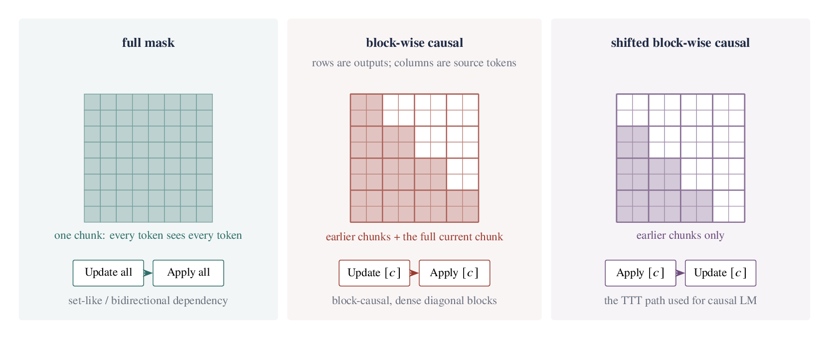
update/apply order as a dependency-mask design choice. Filled cells mean that an output token can depend on a source token. The dense diagonal blocks in the middle panel are bidirectional within each chunk; shifting the update after the apply removes those diagonal blocks.With one full-sequence chunk, update → apply gives every query access to the entire input. Repeating update → apply chunk by chunk gives a block-wise causal mask: an output sees all earlier chunks and all tokens in its current chunk. It is causal between chunks but bidirectional inside each diagonal block. Reversing the order to apply → update shifts the mask by one chunk: the current output reads only fast-weight information written by earlier chunks.
Language modeling shifts TTT, then restores local causality
An autoregressive language model cannot use the dense diagonal blocks above, because an early token would see later tokens from the same chunk. LaCT therefore uses the shifted schedule for its TTT branch:
The output of chunk \(c\) reads a fast weight containing chunks before \(c\); only after that read does the current chunk update the state for future chunks. This avoids future leakage, but it deliberately leaves the TTT branch with no token-level interaction inside the current chunk.
LaCT fills that gap with a parallel causal sliding-window-attention branch. The two branches share QKV projections and their outputs are added:
The two branches have separate jobs. Shifted TTT compresses and retrieves history beyond the local window, while causal sliding-window attention supplies the fine-grained interactions inside the current chunk and its nearby past. The paper chooses an attention window at least as large as the TTT chunk so the union of the two masks has no causal gaps.
The data structure chooses the schedule
It is more useful to organize these choices by which tokens are already valid context when a query is evaluated, rather than by a simple “text” versus “vision” split.
| Task | Chunk choice | TTT schedule | Reason |
|---|---|---|---|
| Language modeling | Configured blocks such as 2K or 4K tokens | apply → update plus causal SWA | Every output must exclude future tokens |
| Novel view synthesis | The full visible input-image set, up to very large token counts | Update from all input tokens, then apply to input and target queries | The input views form an unordered, fully visible context set |
| Autoregressive video diffusion | Groups aligned with several frames | Selective, strided updates from clean chunks; apply to the chunks being denoised | Visual tokens are structured, but future generated content must still remain hidden |
Thus “visual modality” does not automatically mean update → apply. Novel view synthesis can use that order because its input set is already known. Autoregressive video still needs a causal schedule, so clean context chunks write the memory and noisy or current chunks read it without writing future information backward.
Parallel inside a chunk, recurrent across chunks
LaCT does not remove every recurrence. Tokens inside one large chunk can run through the fast-weight network and contribute gradients in parallel, but the updated fast weight is generally handed to the next chunk in order. When one chunk spans multiple devices, context parallelism shards the tokens inside that chunk and combines their update contributions; it does not make dependent chunks independent.
Very large chunks also change the GPU workload. They turn small memory-bound online updates into large PyTorch matrix multiplications, amortize optimizer work, and make a much larger nonlinear fast-weight network practical. The paper uses chunk sizes from thousands of tokens to an entire million-token input set, depending on the task. The chunk size is configurable and chosen to match the task's data structure; it does not necessarily change automatically from one chunk to the next at runtime.
The exact chunkwise DeltaNet algorithm preserves a tokenwise recurrence and changes only how we execute it. LaCT lets every token in a chunk share one pre-update fast weight, combines their learning signal, and chooses an update/apply order that defines the dependency mask. The same word “chunk” therefore names two mathematically different decisions.
update/apply order determines which tokens can influence each output.
References
- [1]
- [2]
- [3]
- [4]
- [5]
- [6]
- [7]
- [8]
- [9]
- [10]
- [11]
- [12]
- [13]